i’d rather have someone put a cigratte in my eye than parse pdfs.
~ BW (very accomplished coder) in a discussion about parsing healthtech pdfs
First, I trust everyone is safe. Second, I haven’t written a SnakeByte in a minute. If you’ve ever wrestled with a PDF that’s more fortress than file, you know, the kind where tables bleed into footnotes, images hide secrets, and your LLM chokes on the chaos, then you will appreciate this one.
Today, we’re diving into MegaParse, an open-source beast from QuivrHQ that’s built to crack open documents like a nutcracker on steroids. It’s optimized for LLM ingestion with zero information loss, turning messy PDFs, DOCXs, and PPTXs into clean, structured gold for your AI overlords. No more “sorry, Dave, I can’t parse that” moments.
If you’ve ever wired up RAG only to discover your PDF tables came out as ASCII i dont know what and your PowerPoints forgot their speaker notes, you’ve met the real villain: lossy parsing. Quivr’s Megaparse is an OSS parser that aims for no-loss conversion across PDFs, DOCX, PPTX, CSV/Excel, shipping markdown you can trust for embeddings and evals. Oh, and let’s not forget EDI specifications. No really.
Read On, Oh Dear Reader.
i stumbled on this gem while hunting for better ways to feed real-world docs into my own RAG experiments. In a world drowning in unstructured data (what is that saying about drowning in data and starving for information? Oh The Megatrends book), MegaParse isn’t just a parser; it’s a precision tool that respects the full spectrum: headers, footers, tables, TOCs, and even images. And get this: it comes in a “vision” mode that ropes in multimodal models like GPT-4o or Claude 3.5 to handle the gnarly stuff. Benchmarks show it smoking the competition with a 0.87 similarity ratio, way ahead of Unstructured's 0.59 or Llama Parser’s measly 0.33. That’s not hype; that’s math saying “this thing gets your docs.”
Why Bother? The Parser Wars Are Real
We’ve all been there: You dump a scanned report into an LLM, and out comes exploding salad. Traditional parsers mangle layouts, drop tables, or hallucinate whitespace where there shouldn’t be any. MegaParse flips the script by prioritizing fidelity no loss, period. It’s fast, free, and plays nice with LangChain, making it a drop-in for anyone building knowledge bases or chatty agents.
Key superpowers:
File Feast: Eats PDFs, DOCX, PPTX, TXT, Excel, CSV – you name it.
Content Clutch: Grabs tables, images, headers/footers without breaking a sweat.
Vision Boost: For the tough nuts, it calls in heavy hitters like GPT-4o to visually dissect pages.
Eval-Ready: Built-in benchmarking scripts to pit it against rivals. (Pro tip: Tweak evaluations/script.py and run it instant flex.)
It’s early days (still cooking table checkers, and structured outputs), but dang if it doesn’t feel like the parser we’ve been waiting for. Open source means you can fork it, fix it, or feast on it. Please be a good steward and contribute back. It is Apache 2.0 license.
Hands-On: Parsing Like a Pro
Let’s get dirty with some code. I’ll walk you through setup and a couple examples. (Assuming Python 3.11+ – because who lives in the past?)
Quick Install & Setup
Fire up your terminal:
pip install megaparse
I trust that wasn’t too difficult.
Ops notes (the stuff you’ll forget at 2am)
Containers: Repo includes Dockerfile and Dockerfile.gpu if you prefer hermetic builds.
System deps: PDFs/images benefit from Poppler and Tesseract; macOS also needs libmagic. Homebrew: brew install poppler tesseract libmagic.
Keys: Vision path needs an LLM key (OpenAI/Anthropic). Plain parser path can run without, depending on your inputs and slap it in a .env file (no keys in the code, boys and girls!):
OPENAI_API_KEY=your_key_here #dont put your OpenAI key for the Anthropic Key
Example 1: Basic Parse: Effortless Extraction
Here’s the no-frills way to crack a PDF. It spits out a structured response ready for your LLM prompt. Ok, so some of you are saying ‘What’s the big deal on PDF Shredding and Parsing?” Well, check my quote at the beginning of this blog. Historically, you had to roll your own regex and then use NLTK, for example.
from megaparse import MegaParse
import json

# Initialize the parser
parser = MegaParse()

# Parse the PDF
response = parser.load("./complex_annual_report_that_no_one_wants_to_read.pdf")

# Pretty-print the output
print(json.dumps(response, indent=2))
Output? A tidy dictionary or list with sections, text, tables all intact. Feed that to your LLM, and watch it hum.
Example2: Parse -> Chunk-> Embed
 pip install megaparse tiktoken numpy sentence-transformers
from megaparse import MegaParse
from sentence_transformers import SentenceTransformer
import tiktoken, textwrap

mp = MegaParse()
doc = mp.load("./docs/board_minutes.pdf")         # -> {"markdown", "metadata", "images"}

# naive chunking by tokens
enc = tiktoken.get_encoding("cl100k_base")
def chunks(markdown, max_tokens=400):
    buf, count = [], 0
    for para in markdown.split("\n\n"):
        tokens = len(enc.encode(para))
        if count + tokens > max_tokens and buf:
            yield "\n\n".join(buf); buf, count = [], 0
        buf.append(para); count += tokens
    if buf: yield "\n\n".join(buf)

model = SentenceTransformer("all-MiniLM-L6-v2")
texts = list(chunks(doc["markdown"]))
embs  = model.encode(texts, convert_to_numpy=True)

print(f"Ingested {len(texts)} chunks; emb shape: {embs.shape}")
In the above example, you will notice tiktoken. tiktoken is a fast open-source Byte Pair Encoding (BPE) tokenizer developed by OpenAI for use with their models. It allows you to convert text strings into tokens (numerical representations) and vice versa, which is crucial for interacting with large language models (LLMs).
Swap in your vector store of choice; the point is the markdown quality gives you cleaner chunks and better recall.
In the above example.:
<N> = how many markdown chunks your PDF becomes with the ~400-token chunker.
384 = embedding size of all-MiniLM-L6-v2.
So if your document yields 12 chunks:
Ingested 12 chunks; emb shape: (12, 384)
Example 3: Vision Mode: When Pixels Get Personal
For docs with wonky scans (anything that uses an identity) or embedded visuals (think human identification or HotDogOrNot), flip to MegaParseVision. It uses a multimodal model to “see” the page, ensuring nothing gets lost in translation.
import os
from langchain_openai import ChatOpenAI
from megaparse.parser.megaparse_vision import MegaParseVision

# Set up your vision model (GPT-4o here; swap for Claude if you're fancy)
model = ChatOpenAI(model="gpt-4o", api_key=os.getenv("OPENAI_API_KEY"))

# Fire up the vision parser
vision_parser = MegaParseVision(model=model)

# Convert with eyes wide open
response = vision_parser.convert("./scanned_presentation.pptx")
print(response)
So, how to read the performance on output:
From their README benchmark (higher is better on their similarity metric):
Use this as a starting point, always test on your corpus (contracts, clinical notes, 10-Qs). They provide a evaluations/script.py hook for plugging in your own comparisons.
NOTE: I didn’t dig into the specifics of the distance similarity functions on how that is derived; however, I am guessing it’s one of the main ones on vector output.
This bad boy achieves that 0.87 benchmark score by visually cross-checking layouts. Pro move: Chain it with LangChain for RAG: parse once, query forever.
The output of the vision parser code using MegaParseVision depends on the input file (in this case, scanned_presentation.pptx) and the specific content within it, as well as the multimodal model used (e.g., GPT-4o).
Expected Output of the Vision Parser Code
The MegaParseVision class in the provided code processes the input file (a PowerPoint presentation, .pptx) using a multimodal model to extract content with high fidelity, including text, tables, images, and layout details. The output is typically a structured Python object (likely a dictionary or list) containing the parsed content, optimized for LLM ingestion. Here’s a breakdown of what you’d generally get:
Structured JSON-like Output: The response from vision_parser.convert(“./scanned_presentation.pptx”) is a structured data format (e.g., a dictionary) with keys representing different elements of the document, such as:
Text: Extracted text from slides, headers, footers, or annotations.
Tables: Structured data from any tables, often as lists or dictionaries representing rows and columns.
Images: Either embedded image data (e.g., base64-encoded) or references to extracted images, depending on configuration.
Metadata: Details like slide numbers, page layout, or document properties.
Visual Elements: For scanned or image-heavy documents, the vision model (e.g., GPT-4o) interprets visual content, so you might get descriptions of charts, diagrams, or other non-text elements.
Example Output Structure
Here’s a hypothetical example of what the output might look like for a simple PowerPoint slide deck with text, a table, and an image:
Comprehensive: Includes all extractable elements (text, tables, images, etc.), leveraging the vision model to interpret scanned or visually complex content.
Structured for LLMs: The output is clean and organized, making it easy to feed into a language model or a RAG pipeline via LangChain.
Vision-Enhanced: Since MegaParseVision uses a multimodal model, it can describe images or interpret layouts that standard text parsers might miss (e.g., text embedded in images or non-standard table formats).
File-Specific: The exact content depends on the .pptx file’s structure. A scanned document might lean more on image descriptions, while a native PPTX might have cleaner text and table data.
Why the Output Varies
The output hinges on:
File Content: A text-heavy PPTX will yield more text fields; a scanned PDF converted to PPTX might emphasize image descriptions.
Model Choice: GPT-4o might prioritize different details compared to Claude 3.5, affecting how visual elements are described.
Configuration: If you’ve tweaked MegaParseVision settings (e.g., via custom prompts or parameters), the output format might differ slightly.
Bonus: API Mode for the Lazy Devs
Hate scripting? Spin up a local server at localhost:8000. Hit the /docs endpoint for Swagger-style bliss coding. Upload files, get parses zero boilerplate.
Wrapping the Byte: Parse Smarter, Not Harder
MegaParse is a reminder that good tools don’t just work; they respect your data. In the LLM era, where garbage in means garbage out, this is your anti-garbage shield. Star it, fork it, build on it and if you’re tweaking those evals, drop me a line on what you find.
NOTE: Benchmarks via their eval script run your own to confirm. No affiliation, just a fan of clean code.
NOTE: On the github “star growth” plot, they use the XKCD Python plotting library. i actually did a SnakeByte on that years ago, love the humor.
Sometimes I tell sky our story. I dont have to say a word. Words are useless in the cosmos; words are useless and absurd.
~ Jess Welles
First, i trust everyone is safe. Second, i am going to write about something that is evolving extremely quickly and we are moving into a world some are calling context engineering. This is beyond prompt engineering. Instead of this just being mainly a python based how-to use a library, i wanted to do some math and some business modeling, thus the name of the blog.
So the more i thought about this i was thinking in terms of how our world is now tokenized. (Remember the token economy ala the word that shall not be named BLOCKCHAIN. Ok, i said it much like saying CandyMan in the movie CandyMan except i dont think anyone will show up if you say blockchain five times).
The old days of crafting clever prompts are fading fast, some say prompting is obsolete. The future isn’t about typing the perfect input; it’s about engineering the entire context in which AI operates and feeding that back into the evolving system. This shift is a game-changer, moving us from toy demos to real-world production systems where AI can actually deliver on scale.
Prompt Engineering So Last Month
Think about it: prompts might dazzle in a controlled demo, but they crumble when faced with the messy reality of actual work. Most AI agents don’t fail because their underlying models are weak—they falter because they don’t see enough of the window and aperture, if you will, is not wide enough. They lack the full situational awareness needed to navigate complex tasks. That’s where context engineering steps in as the new core skill, the backbone of getting AI to handle real jobs effectively.
Words Have Meanings.
~ Dr. Mathew Aldridge
So, what does context engineering mean? It’s a holistic approach to feeding AI the right information at the right time, beyond just a single command. It starts with system prompts that shape the agent’s behavior and voice, setting the tone for how it responds. Then there’s user intent, which frames the actual goalnot just what you ask, but why you’re asking it. Short-term memory keeps multi-step logic and dialogue history alive, while long-term memory stores facts, preferences, and learnings for consistency. Retrieval-Augmented Generation (RAG) pulls in relevant data from APIs, databases, and documents, ensuring the agent has the latest context. Tool availability empowers agents to act not just answer by letting them execute tasks. Finally, structured outputs ensure responses are usable, cutting the fluff and delivering actionable results.
Vertically Trained Horizontally Chained
This isn’t theory; platforms like LangChain and Anthropic are already proving it at scale. They split complex tasks into sub-agents, each with a focused context window to avoid overload. Long chats get compressed via summarization, keeping token limits in check. Sandboxed environments isolate heavy state, preventing crashes, while memory is managed with embeddings, scratchpads, and smart retrieval systems. LangGraph orchestrates these agents with fine-grained control, and LangSmith’s tracing and testing tools evaluate every context tweak, ensuring reliability. It’s a far cry from the old string-crafting days of prompting.
Prompting involved crafting a response with a well-worded sentence. Context engineering is the dynamic design of systems, building full-stack pipelines that provide AI with the right input when it matters. This is what turns a flashy demo into a production-ready product. The magic happens not in the prompt, but in the orchestrated context that surrounds it. As we move forward, mastering this skill will distinguish innovators from imitators, enabling AI to solve real-world problems with precision and power. People will look at you quizzically. In this context, tokens are the food for Large Language Models and are orthogonal to tokens in a blockchain economy.
Slide The Transformers
Which brings us to the evolution of long-context transformers, examining key players, technical concepts, and business implications. NOTE: Even back in the days of the semantic web it was about context.
Foundation model development has entered a new frontier not just of model size, but of memory scale. We’re witnessing the rise of long-context transformers: architectures capable of handling hundreds of thousands and even millions of tokens in a single pass.
This shift is not cosmetic; it alters the fundamental capabilities and business models of LLM platforms. First, i’ll analyze the major players, their long-term strategies, and then we will run through some mathematical architecture powering these transformations. Finally getting down to the Snake Language on basic function implementations for very simple examples.
Company
Model
Max Context Length
Transformer Variant
Notable Use Case
Google
Gemini 1.5 Pro
2M tokens
Mixture-of-Experts + RoPE
Context-rich agent orchestration
OpenAI
GPT-4 Turbo
128k tokens
LLM w/ windowed attention
ChatGPT + enterprise workflows
Anthropic
Claude 3.5 Sonnet
200k tokens
Constitutional Sparse Attention
Safety-aligned memory agents
Magic.dev
LTM-2-Mini
100M tokens
Segmented Recurrence w/ Cache
Codebase-wide comprehension
Meta
Llama 4 Scout
10M tokens
On-device, efficient RoPE
Edge + multimodal inference
Mistral
Mistral Large 2
128k tokens
Sliding Window + Local Attention
Generalist LLM APIs
DeepSeek
DeepSeek V3
128k tokens
Block Sparse Transformer
Multilingual document parsing
IBM
Granite Code/Instruct
128k tokens
Optimized FlashAttention-2
Code generation & compliance
The Matrix Of The Token Grid Arms Race
Redefining Long Context
Here is my explanation and blurb that i researched on each of these:
Google – Gemini 1.5 Pro (2M tokens, Mixture-of-Experts + RoPE) Google’s Gemini 1.5 Pro is a heavyweight, handling 2 million tokens with a clever mix of Mixture-of-Experts and Rotary Positional Embeddings. It shines in context-rich agent orchestration, seamlessly managing complex, multi-step tasks across vast datasets—perfect for enterprise-grade automation.
OpenAI – GPT-4 Turbo (128k tokens, LLM w/ windowed attention) OpenAI’s GPT-4 Turbo packs 128k tokens into a windowed attention framework, making it a go-to for ChatGPT and enterprise workflows. Its strength lies in balancing performance and accessibility, delivering reliable responses for business applications with moderate context needs.
Anthropic – Claude 3.5 Sonnet (200k tokens, Constitutional Sparse Attention) Anthropic’s Claude 3.5 Sonnet offers 200k tokens with Constitutional Sparse Attention, prioritizing safety and alignment. It’s a standout for memory agents, ensuring secure, ethical handling of long conversations—a boon for sensitive industries like healthcare or legal.
Magic.dev – LTM-2-Mini (100M tokens, Segmented Recurrence w/ Cache) Magic.dev’s LTM-2-Mini pushes the envelope with 100 million tokens, using Segmented Recurrence and caching for codebase-wide comprehension. This beast is ideal for developers, retaining entire project histories to streamline coding and debugging at scale.
Meta – Llama 4 Scout (10M tokens, On-device, efficient RoPE) Meta’s Llama 4 Scout brings 10 million tokens to the edge with efficient RoPE, designed for on-device use. Its multimodal inference capability makes it a favorite for privacy-focused applications, from smart devices to defense systems, without cloud reliance.
Mistral – Mistral Large 2 (128k tokens, Sliding Window + Local Attention) Mistral Large 2 handles 128k tokens with Sliding Window and Local Attention, offering a versatile generalist LLM API. It’s a solid choice for broad applications, providing fast, efficient responses for developers and businesses alike.
DeepSeek – DeepSeek V3 (128k tokens, Block Sparse Transformer) DeepSeek V3 matches 128k tokens with a Block Sparse Transformer, excelling in multilingual document parsing. Its strength lies in handling diverse languages and formats, making it a go-to for global content analysis and translation tasks.
IBM – Granite Code/Instruct (128k tokens, Optimized FlashAttention-2) IBM’s Granite Code/Instruct leverages 128k tokens with Optimized FlashAttention-2, tailored for code generation and compliance. It’s a powerhouse for technical workflows, ensuring accurate, regulation-aware outputs for developers and enterprises.
Each of these companies is carving out their own window of context and capabilities for the tokens arms race. So what are some of the basic mathematics at work here for long context?
i’ll integrate Python code to illustrate key architectural ideas (RoPE, Sparse Attention, MoE, Sliding Window) and business use cases (MaaS, Agentic Platforms), using libraries like NumPy, PyTorch, and a mock agent setup. These examples will be practical and runnable in a Jupyter environment.
Rotary Positional Embeddings (RoPE) Extensions
Rotary Positional Embeddings (RoPE) is a technique for incorporating positional information into Transformer-based Large Language Models (LLMs). Unlike traditional methods that add positional vectors, RoPE encodes absolute positions with a rotation matrix and explicitly includes relative position dependency within the self-attention mechanism. This approach enhances the model’s ability to handle longer sequences and better understand token interactions across larger contexts.
The core idea behind RoPE involves rotating the query and key vectors within the attention mechanism based on their positions in the sequence. This rotation encodes positional information and affects the dot product between query and key vectors, which is crucial for attention calculations.
To allow for arbitrarily long context, models generalize RoPE using scaling factors and interpolation. Here is the set of basic equations:
where , extended by interpolation.
Here is some basic code implementing this process:
import numpy as np
import torch

def apply_rope(input_seq, dim=768, max_seq_len=1000000):
    """
    Apply Rotary Positional Embeddings (RoPE) to input sequence.
    Args:
        input_seq (torch.Tensor): Input tensor of shape (batch_size, seq_len, dim)
        dim (int): Model dimension (must be even)
        max_seq_len (int): Maximum sequence length for precomputing positional embeddings
    Returns:
        torch.Tensor: Input with RoPE applied, same shape as input_seq
    """
    batch_size, seq_len, dim = input_seq.shape
    assert dim % 2 == 0, "Dimension must be even for RoPE"

    # Compute positional frequencies for half the dimension
    theta = 10000 ** (-2 * np.arange(0, dim//2, 1) / (dim//2))
    pos = np.arange(seq_len)
    pos_emb = pos[:, None] * theta[None, :]
    pos_emb = np.stack([np.cos(pos_emb), np.sin(pos_emb)], axis=-1)  # Shape: (seq_len, dim//2, 2)
    pos_emb = torch.tensor(pos_emb, dtype=torch.float32).view(seq_len, -1)  # Shape: (seq_len, dim)

    # Reshape and split input for RoPE
    x = input_seq  # Keep original shape (batch_size, seq_len, dim)
    x_reshaped = x.view(batch_size, seq_len, dim//2, 2).transpose(2, 3)  # Shape: (batch_size, seq_len, 2, dim//2)
    x_real = x_reshaped[:, :, 0, :]  # Real part, shape: (batch_size, seq_len, dim//2)
    x_imag = x_reshaped[:, :, 1, :]  # Imaginary part, shape: (batch_size, seq_len, dim//2)

    # Expand pos_emb for batch dimension and apply RoPE
    pos_emb_expanded = pos_emb[None, :, :].expand(batch_size, -1, -1)  # Shape: (batch_size, seq_len, dim)
    out_real = x_real * pos_emb_expanded[:, :, ::2] - x_imag * pos_emb_expanded[:, :, 1::2]
    out_imag = x_real * pos_emb_expanded[:, :, 1::2] + x_imag * pos_emb_expanded[:, :, ::2]

    # Combine and reshape back to original
    output = torch.stack([out_real, out_imag], dim=-1).view(batch_size, seq_len, dim)
    return output

# Mock input sequence (batch_size=1, seq_len=5, dim=4)
input_tensor = torch.randn(1, 5, 4)
rope_output = apply_rope(input_seq=input_tensor, dim=4, max_seq_len=5)
print("RoPE Output Shape:", rope_output.shape)
print("RoPE Output Sample:", rope_output[0, 0, :])  # Print first token's output
The shape verifies the function’s dimensional integrity, ensuring it’s ready for downstream tasks. The sample gives a glimpse into the transformed token, showing RoPE’s effect. You can compare it to the raw input_tensor[0, 0, :] tto see the rotation (though exact differences depend on position and frequency).see the rotation (though exact differences depend on position and to see the rotation (though exact differences depend on position and frequency).
Sparse Attention Mechanisms:
Sparse attention mechanisms are techniques used in transformer models to reduce computational cost by focusing on a subset of input tokens during attention calculations, rather than considering all possible token interactions. This selective attention process enhances efficiency and allows models to handle longer sequences, making them particularly useful for natural language processing tasks like translation and summarization.
In standard self-attention mechanisms, each token in an input sequence attends to every other token, resulting in a computational complexity that scales quadratically with the sequence length . For long sequences, this becomes computationally expensive. Sparse attention addresses this by selectively attending to a subset of tokens, reducing the computational burden. Complexity drops from to or better using block or sliding windows.
Sparse attention mechanisms achieve this reduction in computation by reducing the number of interactions instead of computing attention scores for all possible token pairs, sparse attention focuses on a smaller, selected set of tokens. The downside is by focusing on a subset of tokens, sparse attention may potentially discard some relevant information, which could negatively impact performance on certain tasks. Also it gets more complex code-wise.
The sparse_attention function implements a simplified attention mechanism with a sliding window mask, mimicking sparse attention patterns used in long-context transformers. It takes query (q), key (k), and value (v) tensors, computes attention scores, applies a mask to limit the attention window, and returns the weighted output. The shape torch.Size([1, 2, 6, 4]) indicates that the output tensor has the same structure as the input v tensor. This is expected because the attention mechanism computes a weighted sum of the value vectors based on the attention scores derived from q and k. The sliding window mask(defined by window_size=3) restricts attention to the current token and the previous 2 tokens (diagonal offset of 1-window_size), but it doesn’t change the output shape it only affects which scores contribute to the weighting. The output retains the full sequence length and head structure, ensuring compatibility with downstream layers in a transformer model. This shape signifies that for each of the 1 batch, 2 heads, and 6 tokens, the output is a 4-dimensional vector, representing the attended features after the sparse attention operation.
Mixture-of-Experts (MoE) + Routing
Mixture-of-Experts (MoE) is a machine learning technique that utilizes multiple specialized neural networks, called “experts,” along with a routing mechanism to process input data. The router, a gating network, determines which experts are most relevant for a given input and routes the data accordingly, activating only those specific experts. This approach allows for increased model capacity and computational efficiency, as only a subset of the model needs to be activated for each input.
Key Components:
Experts: These are individual neural networks, each trained to be effective at processing specific types of data or patterns. They can be simple feedforward networks, or even more complex structures.
Routing/Gating Network:This component acts as a dispatcher, deciding which experts are most appropriate for a given input. It typically uses a learned weighting or probability distribution to select the experts.
This basic definition activates a sparse subset of experts:
(Simulating MoE with 2 of 4 experts):
import torch
import torch.nn as nn

class MoE(nn.Module):
    def __init__(self, num_experts=4, top_k=2):
        super().__init__()
        self.experts = nn.ModuleList([nn.Linear(4, 4) for _ in range(num_experts)])
        self.gate = nn.Linear(4, num_experts)
        self.top_k = top_k

    def forward(self, x):
        scores = self.gate(x)  # (batch, num_experts)
        _, top_indices = scores.topk(self.top_k, dim=-1)  # Select top 2 experts
        output = torch.zeros_like(x)
        for i in range(x.shape[0]):
            for j in top_indices[i]:
                output[i] += self.experts[j](x[i])
        return output / self.top_k

# Mock input (batch=2, dim=4)
x = torch.randn(2, 4)
moe = MoE(num_experts=4, top_k=2)
moe_output = moe(x)
print("MoE Output Shape:", moe_output.shape)
This should give you the output:
MoE Output Shape: torch.Size([2, 4])
The shape torch.Size([2, 4]) indicates that the output tensor has the same batch size and dimension as the input tensor x. This is expected because the MoE applies a linear transformation from each selected expert (all outputting 4-dimensional vectors) and averages them, maintaining the input’s feature space. The Mixture-of-Experts mechanism works by:
Computing scores via self.gate(x), producing a (2, 4) tensor that’s transformed to (2, num_experts) (i.e., (2, 4)).
Selecting the top_k=2 experts per sample using topk, resulting in indices for the 2 best experts out of 4.
Applying each expert’s nn.Linear(4, 4) to the input x[i], summing the outputs, and dividing by top_k to normalize the contribution.
The output represents the averaged transformation of the input by the two most relevant experts for each sample, tailored to the input’s characteristics as determined by the gating function.
Sliding Window + Recurrence for Locality
While A context window in an AI model refers to the amount of information (tokens in text) it can consider at any one time. The Locality emphasizes the importance of data points that are close together in a sequence. In many applications, recent information is more relevant than older information. For example, in conversations, recent dialogue contributes most to a coherent response. The importance of that addition lies in effectively handling long contexts in large language models (LLMs) and optimizing inference. Strategies involve splitting the context into segments and managing the Key-Value (KV) cache using data structures like trees.
Segmenting Context: For very long inputs, the entire context might not fit within the model’s memory or process efficiently as a single unit. Therefore, the context can be divided into smaller, manageable segments or chunks.
KV Cache: During LLM inference, the KV cache stores previously computed “keys” and “values” for tokens in the input sequence. This avoids recomputing attention mechanisms for already processed tokens, speeding up the generation process ergo the terminology.
This code splits context into segments with KV cache trees.
import torch

def sliding_window_recurrence(input_seq, segment_size=3, cache_size=2):
    """
    Apply sliding window recurrence with caching.
    Args:
        input_seq (torch.Tensor): Input tensor of shape (batch_size, seq_len, dim)
        segment_size (int): Size of each segment
        cache_size (int): Size of the cache
    Returns:
        torch.Tensor: Output with recurrence applied
    """
    batch_size, seq_len, dim = input_seq.shape
    output = []
    # Initialize cache with batch dimension
    cache = torch.zeros(batch_size, cache_size, dim)  # Shape: (batch_size, cache_size, dim)

    for i in range(0, seq_len, segment_size):
        segment = input_seq[:, i:i+segment_size]  # Shape: (batch_size, segment_size, dim)
        # Ensure cache and segment dimensions align
        if segment.size(1) < segment_size and i + segment_size <= seq_len:
            segment = torch.cat([segment, torch.zeros(batch_size, segment_size - segment.size(1), dim)], dim=1)
        # Mock recurrence: combine with cache
        combined = torch.cat([cache, segment], dim=1)[:, -segment_size:]  # Take last segment_size
        output.append(combined)
        # Update cache with the last cache_size elements
        cache = torch.cat([cache, segment], dim=1)[:, -cache_size:]

    return torch.cat(output, dim=1)

# Mock input (batch=1, seq_len=6, dim=4)
input_tensor = torch.randn(1, 6, 4)
recurrent_output = sliding_window_recurrence(input_tensor, segment_size=3, cache_size=2)
print("Recurrent Output Shape:", recurrent_output.shape)
The output should be:
Recurrent Output Shape: torch.Size([1, 6, 4])
The shape torch.Size([1, 6, 4]) indicates that the output tensor has the same structure as the input tensor input_tensor. This is intentional, as the function aims to process the entire sequence while applying a recurrent mechanism. Sliding Window Process:
The input sequence (length 6) is split into segments of size 3. With seq_len=6 and segment_size=3, there are 2 full segments (indices 0:3 and 3:6).
Each segment is combined with a cache (size 2) using torch.cat, and the last segment_size elements are kept (e.g., (2+3)=5 elements, sliced to 3).
The loop runs twice, appending segments and torch.cat(output, dim=1) reconstructs the full sequence length of 6.
For the Recurrence Effect the cache (initialized as (1, 2, 4)) carries over information from previous segments, mimicking a recurrent neural network’s memory. The output at each position reflects the segment’s data combined with the cache’s prior context, but the shape remains unchanged because the function preserves the original sequence length. In practical applicability for a long-context model, this output could feed into attention layers, where the recurrent combination enhances positional awareness across segments, supporting lengths like 10M tokens (e.g., Meta’s Llama 4 Scout).
So how do we make money? Here are some business model implications.
MemoryAsAService: MaaS class mocks token storage and retrieval with a cost model. For enterprise search, compliance, and document workflows, long-context models enable models to hold entire datasets in RAM, reducing RAG complexity.
Revenue lever: Metered billing based on tokens stored and tokens retrieved
Agentic Platforms and Contextual Autonomy: (With 10M+ token windows), AI agents can:
Load multiyear project timelines
Track legal/compliance chains of thought
Maintain psychological memory for coaching or therapy
Revenue lever: Subscription for persistent agent state memory
Embedded / Edge LLMs: Pruning the attention mimics on-device optimization.
What are you attentive to and where are you attentive to? This is very important for autonomy systems. Insect-like LLMS? Models uses hardware-tuned attention pruning to run on-device without cloud support.
Revenue lever:
Hardware partnerships (Qualcomm, Apple, etc.)
Private licensing for defense/healthcare
Developer Infrastructure: Codebase Memory tracks repo events. Can Haz Logs? Devops on steroids. Analyize repos based on quality and deployment size.
Revenue lever: Developer SaaS pricing by repo or engineering team size (best fewest ups the revenue per employee and margin).
Magic.dev monetizes 100M-token memory by creating LLM-native IDEs that retain architecture history, unit tests, PRs, and stack traces. Super IDE’s for Context Engineering?
Here are some notional mappings for catalyst:
Business Edge
Mathematical Leverage
Persistent memory
Attention cache, memory layers, LRU gating
Low latency
Sliding windows, efficient decoding
Data privacy
On-device + quantized attention ops
Vertical domain AI
MoE + sparse fine-tuning adapters
Closing
In this token-maximized world, the architectural arms race is becoming a memory computation problem. The firms that master the blend of:
Efficient inference at high context length
Agentic memory persistence
Economically viable context scaling will win not just on benchmark scores, but on unit economics, retention, and defensibility.
In the world of AI business models, context is the new (i couldnt think of a buzzword please help me LazyWebTM)? Also I believe that William Gibson was right. Got More Ram?
Until Then.
#iwishyouwater
Ted ℂ. Tanner Jr. (@tctjr) / X
MUZAK TO BLOG BY: Jesse Welles, Pilgrim. If you havent listened to Jesse Welles you are missing out. He is our present-day Bob Dylan. Look him up on youtube out in the field and under the power lines.
Abandon the urge to simplify everything, to look for formulas and easy answers, and to begin to think multidimensionally, to glory in the mystery and paradoxes of life.
~ Scott Peck
First, i hope everyone is safe. Second, I’m writing a SnakeByte that is very near and dear to my heart, fractals. Which is actually encapsulated in the areas of complexity theory, Fibonacci sequences, and the Golden Ratio, ϕ. The world around Us and Our Universe is teeming with these self-similar geometries. Also, sometime ago, i wrote a blog on the mathematics of Grief and how I thought it was fractal-based, never-ending, ever-evolving, entitled “It’s An Honor To Say Goodbye”.
For example:
Golden Ratio: Appears in fractals as a scaling factor for self-similar structures (e.g., golden spirals, golden triangles) and in the proportions of natural fractals.
Fibonacci Sequence: Manifests in the counting of fractal elements (e.g., spirals in sunflowers, branches in trees) and converges to ϕ, linking to fractal scaling.
Mandelbrot Set: Contains spiral patterns that can approximate ϕ-based logarithmic spirals, especially near the boundary.
Nature and Art: Both fractals and Fibonacci patterns appear in natural growth and aesthetic designs, reflecting universal mathematical principles as well as our own bodies.
Fractals are mesmerizing mathematical objects that exhibit self-similarity, meaning their patterns repeat at different scales. Their intricate beauty and complexity make them a fascinating subject for mathematicians, artists, and programmers alike. In this blog, i’l dive into the main types of fractals and then create an interactive visualization of the iconic Mandelbrot set using Python and Bokeh, complete with adjustable parameters. get ready Oh Dear Readers i went long in the SnakeTooth.
Like What Are Fractals?
A fractal is a geometric shape that can be split into parts, each resembling a smaller copy of the whole. Unlike regular shapes like circles or squares, fractals have a fractional dimension and display complexity at every magnification level. They’re often generated through iterative processes or recursive algorithms, making them perfect for computational exploration.
Fractals have practical applications too, from modeling natural phenomena (like tree branching or mountain ranges) to optimizing antenna designs and generating realistic graphics in movies and games.
Types of Fractals
Fractals come in various forms, each with unique properties and generation methods. Here are the main types:
Geometric Fractals
Geometric fractals are created through iterative geometric rules, where a simple shape is repeatedly transformed. The result is a self-similar structure that looks the same at different scales.
Example: Sierpinski Triangle
Start with a triangle, divide it into four smaller triangles, and remove the central one. Repeat this process for each remaining triangle.
The result is a triangle with an infinite number of holes, resembling a lace-like pattern.
Begin with a straight line, divide it into three parts, and replace the middle part with two sides of an equilateral triangle. Repeat for each segment.
The curve becomes infinitely long while enclosing a finite area.
Properties: Continuous but non-differentiable, infinite perimeter.
Algebraic Fractals
Algebraic fractals arise from iterating complex mathematical functions, often in the complex plane. They’re defined by equations and produce intricate, non-repeating patterns.
Example: Mandelbrot Set (the one you probably have seen)
Defined by iterating the function where and are complex numbers.
Points that remain bounded under iteration form the Mandelbrot set, creating a black region with a colorful, infinitely complex boundary.
Properties: Self-similarity at different scales, chaotic boundary behavior.
Example: Julia Sets
Similar to the Mandelbrot set but defined for a fixed value, with varying across the plane.
Each produces a unique fractal, ranging from connected “fat” sets to disconnected “dust” patterns.
Properties: Diverse shapes, sensitive to parameter changes.
Random Fractals
Random fractals incorporate randomness into their construction, mimicking natural phenomena like landscapes or clouds. They’re less predictable but still exhibit self-similarity.
Example: Brownian Motion
Models the random movement of particles, creating jagged, fractal-like paths.
Used in physics and financial modeling.
Properties: Statistically self-similar, irregular patterns. Also akin to the tail of a reverb. Same type of fractal nature.
Example: Fractal Landscapes
Generated using algorithms like the diamond-square algorithm, producing realistic terrain or cloud textures.
Common in computer graphics for games and simulations.
Strange attractors arise from chaotic dynamical systems, where iterative processes produce fractal patterns in phase space. They’re less about geometry and more about the behavior of systems over time.
Example: Lorenz Attractor
Derived from equations modeling atmospheric convection, producing a butterfly-shaped fractal.
Used to study chaos theory and weather prediction.
Properties: Non-repeating, fractal dimension, sensitive to initial conditions.
Now Let’s Compute Some Complexity
Fractals are more than just pretty pictures. They help us understand complex systems, from the growth of galaxies to the structure of the internet. For programmers, fractals are a playground for exploring algorithms, visualization, and interactivity. Let’s now create an interactive Mandelbrot set visualization using Python and Bokeh, where you can tweak parameters like zoom and iterations to explore its infinite complexity.
The Mandelbrot set is a perfect fractal to visualize because of its striking patterns and computational simplicity. We’ll use Python with the Bokeh library to generate an interactive plot, allowing users to adjust the zoom level and the number of iterations to see how the fractal changes.
Basic understanding of Python and complex numbers.
Code Overview
The code below does the following:
Computes the Mandelbrot set by iterating the function for each point in a grid.
Colors points based on how quickly they escape to infinity (for points outside the set) or marks them black (for points inside).
Uses Bokeh to create a static plot with static parameters.
Uses Bokeh to create a static plot.
Displays the fractal as an image with a color palette.
import numpy as np
from bokeh.plotting import figure, show
from bokeh.io import output_notebook
from bokeh.models import LogColorMapper, LinearColorMapper
from bokeh.palettes import Viridis256
import warnings
warnings.filterwarnings('ignore')

# Enable Bokeh output in Jupyter Notebook
output_notebook()

# Parameters for the Mandelbrot set
width, height = 800, 600  # Image dimensions
x_min, x_max = -2.0, 1.0  # X-axis range
y_min, y_max = -1.5, 1.5  # Y-axis range
max_iter = 100  # Maximum iterations for divergence check

# Create coordinate arrays
x = np.linspace(x_min, x_max, width)
y = np.linspace(y_min, y_max, height)
X, Y = np.meshgrid(x, y)
C = X + 1j * Y  # Complex plane

# Initialize arrays for iteration counts and output
Z = np.zeros_like(C)
output = np.zeros_like(C, dtype=float)

# Compute Mandelbrot set
for i in range(max_iter):
    mask = np.abs(Z) <= 2
    Z[mask] = Z[mask] * Z[mask] + C[mask]
    output += mask

# Normalize output for coloring
output = np.log1p(output)

# Create Bokeh plot
p = figure(width=width, height=height, x_range=(x_min, x_max), y_range=(y_min, y_max),
           title="Mandelbrot Fractal", toolbar_location="above")

# Use a color mapper for visualization
color_mapper = LogColorMapper(palette=Viridis256, low=output.min(), high=output.max())
p.image(image=[output], x=x_min, y=y_min, dw=x_max - x_min, dh=y_max - y_min,
        color_mapper=color_mapper)

# Display the plot
show(p)
When you run in in-line you should see the following:
BokehJS 3.6.0 successfully loaded.
Mandlebrot Fractal with Static Parameters
Now let’s do something a little more interesting and add some adjustable parameters for pan and zoom to explore the complex plane space. i’ll break the sections down as we have to add a JavaScript callback routine due to some funkiness with Bokeh and Jupyter Notebooks.
Ok so first of all, let’s break down the imports:
Ok importLibraries:
numpy for numerical computations (e.g., creating arrays for the complex plane).
bokeh modules for plotting (figure, show), notebook output (output_notebook), color mapping (LogColorMapper), JavaScript callbacks (CustomJS), layouts (column), and sliders (Slider).
The above uses Viridis256 for a color palette for visualizing the fractal. FWIW Bokeh provides us with Matplotlib color palettes. There are 5 types of Matplotlib color palettes Magma, Inferno, Plasma, Viridis, Cividis. Magma is my favorite.
Warnings: Suppressed to avoid clutter from Bokeh or NumPy. (i know treat all warnings as errors).
import numpy as np
from bokeh.plotting import figure, show
from bokeh.io import output_notebook
from bokeh.models import LogColorMapper, ColumnDataSource, CustomJS
from bokeh.palettes import Viridis256
from bokeh.layouts import column
from bokeh.models.widgets import Slider
import warnings
warnings.filterwarnings('ignore')
Next, and this is crucial. The following line configures Bokeh to render plots inline in the Jupyter Notebook:
output_notebook()
Initialize the MandleBrot Set Parameters where:
width, height: Dimensions of the output image (800×600 pixels).
initial_x_min, initial_x_max: Range for the real part of complex numbers (-2.0 to 1.0).
initial_y_min, initial_y_max: Range for the imaginary part of complex numbers (-1.5 to 1.5).
max_iter: Maximum number of iterations to determine if a point is in the Mandelbrot set (controls detail).
These ranges define the initial view of the complex plane, centered around the Mandelbrot set’s most interesting region.
Ok, now here is what took me the most time, and I had to research it because, well, because i must be dense. We need to add a JavaScript Callback for Slider Updates. This code updates the plot’s x and y ranges when sliders change, without recomputing the fractal (for performance). For reference: Javascript Callbacks In Bokeh.
zoom_factor: Scales the view (1.0 = original size, <1 zooms in, >1 zooms out).
x_center: Shifts the real axis center by x_pan.value from the initial center.
y_center: Shifts the imaginary axis center by y_pan.value.
x_width, y_height: Scale the original ranges by zoom_factor.
Updates p.x_range and p.y_range to reposition and resize the view.
The callback triggers whenever any slider’s value changes.
Ok, here is a long explanation which is important for the layout and display to understand what is happening computationally fully:
Layout: Arranges the plot and sliders vertically using column.
Display: Renders the interactive plot in the notebook.
X and Y Axis Labels and Complex Numbers
The x and y axes of the plot represent the real and imaginary parts of complex numbers in the plane where the Mandelbrot set is defined.
X-Axis (Real Part):
Label: Implicitly represents the real component of a complex number .
Range: Initially spans -2.0 to 1.0 (covering the Mandelbrot set’s primary region).
Interpretation: Each x-coordinate corresponds to the real part of a complex number . For example, x=−1.5 x = -1.5 x=−1.5 corresponds to a complex number with real part -1.5 .
Role in Mandelbrot: The real part, combined with the imaginary part, defines the constant in the iterative formula .
Y-Axis (Imaginary Part):
Label: Implicitly represents the imaginary component of a complex number .
Range: Initially spans -1.5 to 1.5 (symmetric to capture the set’s structure).
Interpretation: Each y-coordinate corresponds to the imaginary part (scaled by ). For example, y=0.5 y = 0.5 y=0.5 corresponds to a complex number with imaginary part .
Role in Mandelbrot: The imaginary part contributes to , affecting the iterative behavior.
Complex Plane:
Each pixel in the plot corresponds to a complex number , where is the x-coordinate (real part) and is the y-coordinate (imaginary part).
The Mandelbrot set consists of points where the sequence , remains bounded (doesn’t diverge to infinity).
The color at each pixel reflects how quickly the sequence diverges (or if it doesn’t, it’s typically black).
Slider Effects:
X Pan: Shifts the real part center, moving the view left or right in the complex plane.
Y Pan: Shifts the imaginary part center, moving the view up or down.
Zoom: Scales both real and imaginary ranges, zooming in (smaller zoom_factor) or out (larger zoom_factor). Zooming in reveals finer details of the fractal’s boundary.
Performance: The code uses a JavaScript callback to update the view without recomputing the fractal, which is fast but limits resolution. For high-zoom levels, you’d need to recompute the fractal (not implemented here for simplicity).
Axis Labels: Bokeh doesn’t explicitly label axes as “Real Part” or “Imaginary Part,” but the numerical values correspond to these components. You could add explicit labels using p.xaxis.axis_label = “Real Part” and p.yaxis.axis_label = “Imaginary Part” if desired.
Fractal Detail: The fixed max_iter=100 limits detail at high zoom. For deeper zooms, max_iter should increase, and the fractal should be recomputed. Try adding a timer() function to check compute times.
Ok here is the full listing you can copypasta this into a notebook and run it as is. i suppose i could add gist.
import numpy as np
from bokeh.plotting import figure, show
from bokeh.io import output_notebook
from bokeh.models import LogColorMapper, ColumnDataSource, CustomJS
from bokeh.palettes import Viridis256
from bokeh.layouts import column
from bokeh.models.widgets import Slider
import warnings
warnings.filterwarnings('ignore')
# Enable Bokeh output in Jupyter Notebook
output_notebook()
# Parameters for the Mandelbrot set
width, height = 800, 600 # Image dimensions
initial_x_min, initial_x_max = -2.0, 1.0 # Initial X-axis range
initial_y_min, initial_y_max = -1.5, 1.5 # Initial Y-axis range
max_iter = 100 # Maximum iterations for divergence check
# Function to compute Mandelbrot set
def compute_mandelbrot(x_min, x_max, y_min, y_max, width, height, max_iter):
x = np.linspace(x_min, x_max, width)
y = np.linspace(y_min, y_max, height)
X, Y = np.meshgrid(x, y)
C = X + 1j * Y # Complex plane
Z = np.zeros_like(C)
output = np.zeros_like(C, dtype=float)
for i in range(max_iter):
mask = np.abs(Z) <= 2
Z[mask] = Z[mask] * Z[mask] + C[mask]
output += mask
return np.log1p(output)
# Initial Mandelbrot computation
output = compute_mandelbrot(initial_x_min, initial_x_max, initial_y_min, initial_y_max, width, height, max_iter)
# Create Bokeh plot
p = figure(width=width, height=height, x_range=(initial_x_min, initial_x_max), y_range=(initial_y_min, initial_y_max),
title="Interactive Mandelbrot Fractal", toolbar_location="above")
# Use a color mapper for visualization
color_mapper = LogColorMapper(palette=Viridis256, low=output.min(), high=output.max())
image = p.image(image=[output], x=initial_x_min, y=initial_y_min, dw=initial_x_max - initial_x_min,
dh=initial_y_max - initial_y_min, color_mapper=color_mapper)
# Create sliders for panning and zooming
x_pan_slider = Slider(start=-2.0, end=1.0, value=0, step=0.1, title="X Pan")
y_pan_slider = Slider(start=-1.5, end=1.5, value=0, step=0.1, title="Y Pan")
zoom_slider = Slider(start=0.1, end=3.0, value=1.0, step=0.1, title="Zoom")
# JavaScript callback to update plot ranges
callback = CustomJS(args=dict(p=p, x_pan=x_pan_slider, y_pan=y_pan_slider, zoom=zoom_slider,
initial_x_min=initial_x_min, initial_x_max=initial_x_max,
initial_y_min=initial_y_min, initial_y_max=initial_y_max),
code="""
const zoom_factor = zoom.value;
const x_center = initial_x_min + (initial_x_max - initial_x_min) / 2 + x_pan.value;
const y_center = initial_y_min + (initial_y_max - initial_y_min) / 2 + y_pan.value;
const x_width = (initial_x_max - initial_x_min) * zoom_factor;
const y_height = (initial_y_max - initial_y_min) * zoom_factor;
p.x_range.start = x_center - x_width / 2;
p.x_range.end = x_center + x_width / 2;
p.y_range.start = y_center - y_height / 2;
p.y_range.end = y_center + y_height / 2;
""")
# Attach callback to sliders
x_pan_slider.js_on_change('value', callback)
y_pan_slider.js_on_change('value', callback)
zoom_slider.js_on_change('value', callback)
# Layout the plot and sliders
layout = column(p, x_pan_slider, y_pan_slider, zoom_slider)
# Display the layout
show(layout)
Here is the output screen shot: (NOTE i changed it to Magma256)
Mandlebrot Fractal with Interactive Bokeh Sliders.
So there ya have it. A little lab for fractals. Maybe i’ll extend this code and commit it. As a matter of fact, i should push all the SnakeByte code over the years. That said concerning the subject of Fractals there is a much deeper and longer discussion to be had relating fractals, the golden ratio and the Fibonacci sequences (A sequence where each number is the sum of the two preceding ones: 0, 1, 1, 2, 3, 5, 8, 13, 21…) are deeply interconnected through mathematical patterns and structures that appear in nature, art, and geometry. The very essence of our lives.
Until Then.
#iwishyouwater <- Pavones,CR Longest Left in the Northern Hemisphere. i love it there.
Ted ℂ. Tanner Jr. (@tctjr) / X
MUZAK To Blog By: Arvo Pärt, Für Anna Maria, Spiegel im Spiegel (Mirror In Mirror) very fractal song. it is gorgeous.
References:
Here is a very short list of books on the subject. Ping me as I have several from philosophical to mathematical on said subject.
First as always i hope everyone is safe oh Dear Readers. Secondly, i am going to write about something that i have been pondering for quite some time, probably close to two decades.
What i call Religion Of Warez (ROWZ).
This involves someone who i hold in the highest regard YOU the esteemed developer.
Marc Andreeson famously said “Software Is Eating The Word”. Here is the original blog:
There is a war going on for your attention. There is a war going on for your thumb typing. There is a war going on for your viewership. There is a war going on for your selfies. There is a war going on for your emoticons. There is a war going on for github pull requests.
There is a war going on for the output of your prompting.
We have entered into The Great Cognitive Artificial Intelligence Arms Race (TGCAIAR) via camps of Large Languge Model foundational model creators.
The ability to deploy the warez needed to wage war on YOU Oh Dear Reader is much more complex from an ideological perspective. i speculate that Software if i may use that term as an entity is a non-theistic religion. Even within the Main Tabernacle of Software (MTOS) there are various fissures of said religions whether it be languages, architectures or processes.
Let us head over to the LazyWebTM and do a cursory search and see what we find[1] concerning some comparison numbers for religions and software languages.
In going to wikipedia we find:
According to some estimates, there are roughly 4,200 religions, churches, denominations, religious bodies, faith groups, tribes, cultures, movements, ultimate concerns, which at some point in the future will be countless.
Wikipedia
Worldwide, more than eight-in-ten people identify with a religious group. i suppose even though we don’t like to be categorized, we like to be categorized as belonging to a particular sect. Here is a telling graphic:
Let us map this to just computer languages. Just how many computer languages are there? i guessed 6000 in aggregate. There are about 700 main programming languages, including esoteric coding languages. From what i can ascertain some only list notable languages add up to 245 languages. Another list called HOPL, which claims to include every programming language ever to exist, puts the total number of programming languages at 8,945.
So i wasn’t that far off.
Why so much kerfuffle on languages? For those that have ever had a language discussion, did it feel like you were discussing religion? Hmmmm?
Hey, my language does automatic heap management. Why are you messing with memory allocation via this dumb thing called pointers?
The Art of Computer Programming is mapping an idea into a binary computational translation (classical computing rates apply). This process is highly inefficient compared to having binary-to-binary discussions[2]. Note we are not even considering architectures or methods in this mapping. Let us keep it at English to binary representation. What is the dimensionality reduction for that mapping? What is lost in translation?
As i always like to do i refer to Miriam Webster Dictionary. It holds a soft spot in my heart strings as i used to read it in grade school. (Yes i read the dictionary…)
Religion: Noun
re·li·gion (ruh·li·jen)
: a cause, principle, or system of beliefs held to with ardor and faith
Well, now, Dear Reader, the proverbial plot thickens. A System of Beliefs held to faith. Nowadays, religion is utilized as a concept today applied for a genus of social formations that includes several members, a type of which there are many tokens or facets.
If this is, in fact, the case, I will venture to say that Software could be considered a Religion.
One must then ask? Is there “a model” to the madness? Do we go the route of the core religions? Would we dare say the Belief System Of The Warez[3] be included as a prominent religion?
Symbols Of The World Religions
I have said several times and will continue to say that Software is one of the greatest human endeavors of all time. It is at the essence of ideas incarnate.
It has been said that if you adopt the science, you adopt the ideology. Such hatred or fear of science has always been justified in the name of some ideology or other.
If we take this as the undertone for many new aspects of software, we see that the continuum of mind varies within the perception of the universe by which we are affected by said software. It is extremely canonical and first order.
Most often, we anthropomorphize most things and our software is no exception. It is as though it were an entity or even a thing in the most straightforward cases. It is, in fact, neither. It is just information imputed upon our minds via probabilistic models via non convex optimization methods. It is as if it was a Rorschach test that allowed many people to project their own meaning onto it (sound familiar?).
Let me say this a different way. With the advent of ChatGPT we seem to desire IT to be alive or reason somehow someway yet we don’t want it to turn into the terminator.
Stock market predictions – YES
Terminator – NO.
The Thou Shalts Will Kill You
~ Joseph Campbell
Now we are entering a time very quickly where we have “agentic” based large language models that can be scripted for specific tasks and then chained together to perform multiple tasks.
Now we have large language models distilling information gleaned from other LLMs. Who’s peanut butter is in the chocolate? Is there a limit of growth here for information? Asymptotic token computation if you will?
We are nowhere near the end of writing the Religion Of Warez (ROWZ) sacred texts compared to the Bible, Sutras, Vedas, the Upanishads, and the Bhagavad Gita, Quran, Agamas, Torah, Tao Te Ching or Avesta, even the Satanic Bible. My apologies if i left your special tome out it wasn’t on purpose. i could have listed thousands. BTW for reference there is even a religion called the Partridge Family Temple. The cult’s members believe the characters are archetypal gods and goddesses.
In fact we have just begun to author the Religion Of Warez (ROWZ) sacred text. The next chapters are going be accelerated and written via generative adversarial networks, stable fusion and reinforcement learning transformer technologies.
Which, then, one must ask which Diety are YOU going to choose?
i wrote a little stupid python script to show relationships of coding languages based on dates for the main ones. Simple key value stuff. All hail the gods K&R for creating C.
import networkx as nx
import matplotlib.pyplot as plt

def create_language_graph():
    G = nx.DiGraph()

    # Nodes (Programming languages with their release years)
    languages = {
        "Fortran": 1957, "Lisp": 1958, "COBOL": 1959, "ALGOL": 1960,
        "C": 1972, "Smalltalk": 1972, "Prolog": 1972, "ML": 1973,
        "Pascal": 1970, "Scheme": 1975, "Ada": 1980, "C++": 1983,
        "Objective-C": 1984, "Perl": 1987, "Haskell": 1990, "Python": 1991,
        "Ruby": 1995, "Java": 1995, "JavaScript": 1995, "PHP": 1995,
        "C#": 2000, "Scala": 2003, "Go": 2009, "Rust": 2010,
        "Common Lisp": 1984
    }

    # Adding nodes
    for lang, year in languages.items():
        G.add_node(lang, year=year)

    # Directed edges (influences between languages)
    edges = [
        ("Fortran", "C"), ("Lisp", "Scheme"), ("Lisp", "Common Lisp"),
        ("ALGOL", "Pascal"), ("ALGOL", "C"), ("C", "C++"), ("C", "Objective-C"),
        ("C", "Go"), ("C", "Rust"), ("Smalltalk", "Objective-C"),
        ("C++", "Java"), ("C++", "C#"), ("ML", "Haskell"), ("ML", "Scala"),
        ("Scheme", "JavaScript"), ("Perl", "PHP"), ("Python", "Ruby"),
        ("Python", "Go"), ("Java", "Scala"), ("Java", "C#"), ("JavaScript", "Rust")
    ]

    # Adding edges
    G.add_edges_from(edges)

    return G

def visualize_graph(G):
    plt.figure(figsize=(12, 8))
    pos = nx.spring_layout(G, seed=42)
    years = nx.get_node_attributes(G, 'year')

    # Color nodes based on their release year
    node_colors = [plt.cm.viridis((years[node] - 1950) / 70) for node in G.nodes]

    nx.draw(G, pos, with_labels=True, node_color=node_colors, edge_color='gray',
            node_size=3000, font_size=10, font_weight='bold', arrows=True)

    plt.title("Programming Language Influence Graph")
    plt.show()

if __name__ == "__main__":
    G = create_language_graph()
    visualize_graph(G)
Programming Relationship Diagram
So, folks, let me know what you think. I am considering authoring a much longer paper comparing behaviors, taxonomies and the relationship between religions and software.
i would like to know if you think this would be a worthwhile piece?
Until Then,
#iwishyouwater <- Banzai Pipeline January 2023. Amazing.
@tctjr
MUZAK TO BLOG BY: Baroque Ensemble Of Vienna – “Classical Legends of Baroque”. i truly believe i was born in the wrong century when i listen to this level of music. Candidly J.S. Bach is by far my favorite composer going back to when i was in 3rd grade. BRAVO! Stupdendum Perficientur!
[1] Ever notice that searching is not finding? i prefer finding. Someone needs to trademark “Finding Not Searching” The same vein as catching ain’t fishing.
[2] Great paper from OpenAI on just this subject: two agents having a discussion (via reinforcement learning) : https://openai.com/blog/learning-to-communicate/ (more technical paper click HERE)
[3] For a great read i refer you to the The Ware Tetralogy by Rudy Rucker: Software (1982), Wetware (1988), Freeware (1997), Realware (2000)
[4] When the words “software” and “engineering” were first put together [Naur and Randell 1968] it was not clear exactly what the marriage of the two into the newly minted term really meant. Some people understood that the term would probably come to be defined by what our community did and what the world made of it. Since those days in the late 1960’s a spectrum of research and practice has been collected under the term.
~ Professor Benard Widrow (inventor of the LMS algorithm)
Hello Folks! As always, i hope everyone is safe. i also hope everyone had a wonderful holiday break with food, family, and friends.
The first SnakeByte of the new year involves a subject near and dear to my heart: Optimization.
The quote above was from a class in adaptive signal processing that i took at Stanford from Professor Benard Widrow where he talked about how almost everything is a gradient type of optimization and “In Life We Are Always Optimizing.”. Incredibly profound if One ponders the underlying meaning thereof.
So why optimization?
Well glad you asked Dear Reader. There are essentially two large buckets of optimization: Convex and Non Convex optimization.
Convex optimization is an optimization problem has a single optimal solution that is also the global optimal solution. Convex optimization problems are efficient and can be solved for huge issues. Examples of convex optimization include maximizing stock market portfolio returns, estimating machine learning model parameters, and minimizing power consumption in electronic circuits.
Non-convex optimization is an optimization problem can have multiple locally optimal points, and it can be challenging to determine if the problem has no solution or if the solution is global. Non-convex optimization problems can be more difficult to deal with than convex problems and can take a long time to solve. Optimization algorithms like gradient descent with random initialization and annealing can help find reasonable solutions for non-convex optimization problems.
You can determine if a function is convex by taking its second derivative. If the second derivative is greater than or equal to zero for all values of x in an interval, then the function is convex. Ah calculus 101 to the rescue.
Caveat Emptor, these are very broad mathematically defined brush strokes.
So why do you care?
Once again, Oh Dear Reader, glad you asked.
Non-convex optimization is fundamentally linked to how neural networks work, particularly in the training process, where the network learns from data by minimizing a loss function. Here’s how non-convex optimization connects to neural networks:
A loss function is a global function for convex optimization. A “loss landscape” in a neural network refers to representation across the entire parameter space or landscape, essentially depicting how the loss value changes as the network’s weights are adjusted, creating a multidimensional surface where low points represent areas with minimal loss and high points represent areas with high loss; it allows researchers to analyze the geometry of the loss function to understand the training process and potential challenges like local minima. To note the weights can be millions, billions or trillions. It’s the basis for the cognitive AI arms race, if you will.
The loss function in neural networks, measures the difference between predicted and true outputs, is often a highly complex, non-convex function. This is due to:
The multi-layered structure of neural networks, where each layer introduces non-linear transformations and the high dimensionality of the parameter space, as networks can have millions, billions or trillions of parameters (weights and biases vectors).
As a result, the optimization process involves navigating a rugged loss landscape with multiple local minima, saddle points, and plateaus.
Optimization Algorithms in Non-Convex Settings
Training a neural network involves finding a set of parameters that minimize the loss function. This is typically done using optimization algorithms like gradient descent and its variants. While these algorithms are not guaranteed to find the global minimum in a non-convex landscape, they aim to reach a point where the loss is sufficiently low for practical purposes.
This leads to the latest SnakeBtye[18]. The process of optimizing these parameters is often called hyperparameter optimization. Also, relative to this process, designing things like aircraft wings, warehouses, and the like is called Multi-Objective Optimization, where you have multiple optimization points.
As always, there are test cases. In this case, you can test your optimization algorithm on a function called The Himmelblau’s function. The Himmelblau Function was introduced by David Himmelblau in 1972 and is a mathematical benchmark function used to test the performance and robustness of optimization algorithms. It is defined as:
Using Wolfram Mathematica to visualize this function (as i didn’t know what it looked like…) relative to solving for :
Wolfram Plot Of The Himmelblau Function
This function is particularly significant in optimization and machine learning due to its unique landscape, which includes four global minima located at distinct points. These minima create a challenging environment for optimization algorithms, especially when dealing with non-linear, non-convex search spaces. Get the connection to large-scale neural networks? (aka Deep Learnin…)
The Himmelblau’s function is continuous and differentiable, making it suitable for gradient-based methods while still being complex enough to test heuristic approaches like genetic algorithms, particle swarm optimization, and simulated annealing. The function’s four minima demand algorithms to effectively explore and exploit the gradient search space, ensuring that solutions are not prematurely trapped in local optima.
Researchers use it to evaluate how well an algorithm navigates a multi-modal surface, balancing exploration (global search) with exploitation (local refinement). Its widespread adoption has made it a standard in algorithm development and performance assessment.
Several types of libraries exist to perform Multi-Objective or Parameter Optimization. This blog concerns one that is extremely flexible, called OpenMDAO.
What Does OpenMDAO Accomplish, and Why Is It Important?
OpenMDAO (Open-source Multidisciplinary Design Analysis and Optimization) is an open-source framework developed by NASA to facilitate multidisciplinary design, analysis, and optimization (MDAO). It provides tools for integrating various disciplines into a cohesive computational framework, enabling the design and optimization of complex engineering systems.
Key Features of OpenMDAO Integration:
OpenMDAO allows engineers and researchers to couple different models into a unified computational graph, such as aerodynamics, structures, propulsion, thermal systems, and hyperparameter machine learning. This integration is crucial for studying interactions and trade-offs between disciplines.
Automatic Differentiation:
A standout feature of OpenMDAO is its support for automatic differentiation, which provides accurate gradients for optimization. These gradients are essential for efficient gradient-based optimization techniques, particularly in high-dimensional design spaces. Ah that calculus 101 stuff again.
It supports various optimization methods, including gradient-based and heuristic approaches, allowing it to handle linear and non-linear problems effectively.
By making advanced optimization techniques accessible, OpenMDAO facilitates cutting-edge research in system design and pushes the boundaries of what is achievable in engineering.
Lo and Behold! OpenMDAO itself is a Python library! It is written in Python and designed for use within the Python programming environment. This allows users to leverage Python’s extensive ecosystem of libraries while building and solving multidisciplinary optimization problems.
So i had the idea to use and test OpenMDAO on The Himmelblau function. You might as well test an industry-standard library on an industry-standard function!
First things first, pip install or anaconda:
>> pip install 'openmdao[all]'
Next, being We are going to be plotting stuff within JupyterLab i always forget to enable it with the majik command:
## main code
%matplotlib inline
Ok lets get to the good stuff the code.
# add your imports here:
import numpy as np
import matplotlib.pyplot as plt
from openmdao.api import Problem, IndepVarComp, ExecComp, ScipyOptimizeDriver
# NOTE: the scipy import

# Define the OpenMDAO optimization problem - almost like self.self
prob = Problem()

# Add independent variables x and y and make a guess of X and Y:
indeps = prob.model.add_subsystem('indeps', IndepVarComp(), promotes_outputs=['*'])
indeps.add_output('x', val=0.0)  # Initial guess for x
indeps.add_output('y', val=0.0)  # Initial guess for y

# Add the Himmelblau objective function. See the equation from the Wolfram Plot?
prob.model.add_subsystem('obj_comp', ExecComp('f = (x**2 + y - 11)**2 + (x + y**2 - 7)**2'), promotes_inputs=['x', 'y'], promotes_outputs=['f'])

# Specify the optimization driver and eplison error bounbs.  ScipyOptimizeDriver wraps the optimizers in *scipy.optimize.minimize*. In this example, we use the SLSQP optimizer to find the minimum of the "Paraboloid" type optimization:
prob.driver = ScipyOptimizeDriver()
prob.driver.options['optimizer'] = 'SLSQP'
prob.driver.options['tol'] = 1e-6

# Set design variables and bounds
prob.model.add_design_var('x', lower=-10, upper=10)
prob.model.add_design_var('y', lower=-10, upper=10)

# Add the objective function Himmelblau via promotes.output['f']:
prob.model.add_objective('f')

# Setup and run the problem and cross your fingers:
prob.setup()
prob.run_driver()
So this optimized the minima of the function relative to the bounds of and and .
Now, lets look at the cool eye candy in several ways:
# Retrieve the optimized values
x_opt = prob['x']
y_opt = prob['y']
f_opt = prob['f']

print(f"Optimal x: {x_opt}")
print(f"Optimal y: {y_opt}")
print(f"Optimal f(x, y): {f_opt}")

# Plot the function and optimal point
x = np.linspace(-6, 6, 400)
y = np.linspace(-6, 6, 400)
X, Y = np.meshgrid(x, y)
Z = (X**2 + Y - 11)**2 + (X + Y**2 - 7)**2

plt.figure(figsize=(8, 6))
contour = plt.contour(X, Y, Z, levels=50, cmap='viridis')
plt.clabel(contour, inline=True, fontsize=8)
plt.scatter(x_opt, y_opt, color='red', label='Optimal Point')
plt.title("Contour Plot of f(x, y) with Optimal Point")
plt.xlabel("x")
plt.ylabel("y")
plt.legend()
plt.colorbar(contour)
plt.show()
Now, lets try something that looks a little more exciting:
import numpy as np
import matplotlib.pyplot as plt

# Define the function
def f(x, y):
    return (x**2 + y - 11)**2 + (x + y**2 - 7)**2

# Generate a grid of x and y values
x = np.linspace(-6, 6, 500)
y = np.linspace(-6, 6, 500)
X, Y = np.meshgrid(x, y)
Z = f(X, Y)

# Plot the function
plt.figure(figsize=(8, 6))
plt.contourf(X, Y, Z, levels=100, cmap='magma')  # Gradient color
plt.colorbar(label='f(x, y)')
plt.title("Plot of f(x, y) = (x² + y - 11)² + (x + y² - 7)²")
plt.xlabel("x")
plt.ylabel("y")
plt.show()
That is cool looking.
Ok, lets take this even further:
We can compare it to the Wolfram Function 3D plot:
from mpl_toolkits.mplot3d import Axes3D

# Create a 3D plot
fig = plt.figure(figsize=(10, 8))
ax = fig.add_subplot(111, projection='3d')

# Plot the surface
ax.plot_surface(X, Y, Z, cmap='magma', edgecolor='none', alpha=0.9)

# Labels and title
ax.set_title("3D Plot of f(x, y) = (x² + y - 11)² + (x + y² - 7)²")
ax.set_xlabel("x")
ax.set_ylabel("y")
ax.set_zlabel("f(x, y)")

plt.show()
Which gives you a 3D plot of the function:
3D Plot of f(x, y) = (x² + y – 11)² + (x + y² – 7)²
While this was a toy example for OpenMDAO, it is also a critical tool for advancing multidisciplinary optimization in engineering. Its robust capabilities, open-source nature, and focus on efficient computation of derivatives make it invaluable for researchers and practitioners seeking to tackle the complexities of modern system design.
i hope you find it useful.
Until Then,
#iwishyouwater <- The EDDIE – the most famous big wave contest ran this year. i saw it on the beach in 2004 and got washed across e rivermouth on a 60ft clean up set that washed out the river.
Who told you to attack the machines, you fools? Without them you’ll all die!!
~ Grot, the Guardian of the Heart Machine
First, as always, Oh Dear Reader, i hope you are safe. There are many unsafe places in and around the world in this current time. Second, this blog is a SnakeByte[] based on something that i knew about but had no idea it was called this by this name.
Third, relative to this, i must confess, Oh, Dear Reader, i have a disease of the bibliomaniac kind. i have an obsession with books and reading. “They” say that belief comes first, followed by admission. There is a Japanese word that translates to having so many books you cannot possibly read them all. This word is tsundoku. From the website (if you click on the word):
“Tsundoku dates from the Meiji era, and derives from a combination of tsunde-oku (to let things pile up) and dokusho (to read books). It can also refer to the stacks themselves. Crucially, it doesn’t carry a pejorative connotation, being more akin to bookworm than an irredeemable slob.”
Thus, while perusing a math-related book site, i came across a monograph entitled “The Metropolis Algorithm: Theory and Examples” by C Douglas Howard [1].
i was intrigued, and because it was 5 bucks (Side note: i always try to buy used and loved books), i decided to throw it into the virtual shopping buggy.
Upon receiving said monograph, i sat down to read it, and i was amazed to find it was closely related to something I was very familiar with from decades ago. This finally brings us to the current SnakeByte[].
The Metropolis Algorithm is a method in computational statistics used to sample from complex probability distributions. It is a type of Markov Chain Monte Carlo (MCMC) algorithm (i had no idea), which relies on Markov Chains to generate a sequence of samples that can approximate a desired distribution, even when direct sampling is complex. Yes, let me say that again – i had no idea. Go ahead LazyWebTM laugh!
So let us start with how the Metropolis Algorithm and how it relates to Markov Chains. (Caveat Emptor: You will need to dig out those statistics books and a little linear algebra.)
Markov Chains Basics
A Markov Chain is a mathematical system that transitions from one state to another in a state space. It has the property that the next state depends only on the current state, not the sequence of states preceding it. This is called the Markov property. The algorithm was introduced by Metropolis et al. (1953) in a Statistical Physics context and was generalized by Hastings (1970). It was considered in the context of image analysis (Geman and Geman, 1984) and data augmentation (Tanner (I’m not related that i know of…) and Wong, 1987). However, its routine use in statistics (especially for Bayesian inference) did not take place until Gelfand and Smith (1990) popularised it. For modern discussions of MCMC, see e.g. Tierney (1994), Smith and Roberts (1993), Gilks et al. (1996), and Roberts and Rosenthal (1998b).
Ergo, the name Metropolis-Hastings algorithm. Once again, i had no idea.
Anyhow,
A Markov Chain can be described by a set of states and a transition matrix , where each element represents the probability of transitioning from state to state .
Provide The Goal: Sampling from a Probability Distribution
In many applications (e.g., statistical mechanics, Bayesian inference, as mentioned), we are interested in sampling from a complex probability distribution . This distribution might be difficult to sample from directly, but we can use a Markov Chain to create a sequence of samples that, after a certain period (called the burn-in period), will approximate .
Ok Now: The Metropolis Algorithm
The Metropolis Algorithm is one of the simplest MCMC algorithms to generate samples from . It works by constructing a Markov Chain whose stationary distribution is the desired probability distribution . A stationary distribution is a probability distribution that remains the same over time in a Markov chain. Thus it can describe the long-term behavior of a chain, where the probabilities of being in each state do not change as time passes. (Whatever time is, i digress.)
The key steps of the algorithm are:
Initialization
Start with an initial guess , a point in the state space. This point can be chosen randomly or based on prior knowledge.
Proposal Step
From the current state , propose a new state using a proposal distribution , which suggests a candidate for the next state. This proposal distribution can be symmetric (e.g., a normal distribution centered at ) or asymmetric.
Acceptance Probability
Calculate the acceptance probability for moving from the current state to the proposed state :
In the case where the proposal distribution is symmetric (i.e., , the formula simplifies to:
Acceptance or Rejection
Generate a random number from a uniform distribution If , accept the proposed state , i.e., . If , reject the proposed state and remain at the current state, i.e., .
Repeat
Repeat the proposal, acceptance, and rejection steps to generate a Markov Chain of samples.
Convergence and Stationary Distribution:
Over time, as more samples are generated, the Markov Chain converges to a stationary distribution. The stationary distribution is the target distribution , meaning the samples generated by the algorithm will approximate more closely as the number of iterations increases.
Applications:
The Metropolis Algorithm is widely used in various fields such as Bayesian statistics, physics (e.g., in the simulation of physical systems), machine learning, and finance. It is especially useful for high-dimensional problems where direct sampling is computationally expensive or impossible.
Key Features of the Metropolis Algorithm:
Simplicity: It’s easy to implement and doesn’t require knowledge of the normalization constant of , which can be difficult to compute.
Flexibility: It works with a wide range of proposal distributions, allowing the algorithm to be adapted to different problem contexts.
Efficiency: While it can be computationally demanding, the algorithm can provide high-quality approximations to complex distributions with well-chosen proposals and sufficient iterations.
The Metropolis-Hastings Algorithm is a more general version that allows for non-symmetric proposal distributions, expanding the range of problems the algorithm can handle.
Now let us code it up:
i am going to assume the underlying distribution is Gaussian with a time-dependent mean , which changes slowly over time. We’ll use a simple time-series analytics setup to sample this distribution using the Metropolis Algorithm and plot the results. Note: When the target distribution is Gaussian (or close to Gaussian), the algorithm can converge more quickly to the true distribution because of the symmetric smooth nature of the normal distribution.
import numpy as np
import matplotlib.pyplot as plt

# Time-dependent mean function (example: sinusoidal pattern)
def mu_t(t):
    return 10 * np.sin(0.1 * t)

# Target distribution: Gaussian with time-varying mean mu_t and fixed variance
def target_distribution(x, t):
    mu = mu_t(t)
    sigma = 1.0  # Assume fixed variance for simplicity
    return np.exp(-0.5 * ((x - mu) / sigma) ** 2)

# Metropolis Algorithm for time-series sampling
def metropolis_sampling(num_samples, initial_x, proposal_std, time_steps):
    samples = np.zeros(num_samples)
    samples[0] = initial_x

    # Iterate over the time steps
    for t in range(1, num_samples):
        # Propose a new state based on the current state
        x_current = samples[t - 1]
        x_proposed = np.random.normal(x_current, proposal_std)

        # Acceptance probability (Metropolis-Hastings step)
        acceptance_ratio = target_distribution(x_proposed, time_steps[t]) / target_distribution(x_current, time_steps[t])
        acceptance_probability = min(1, acceptance_ratio)

        # Accept or reject the proposed sample
        if np.random.rand() < acceptance_probability:
            samples[t] = x_proposed
        else:
            samples[t] = x_current

    return samples

# Parameters
num_samples = 10000  # Total number of samples to generate
initial_x = 0.0      # Initial state
proposal_std = 0.5   # Standard deviation for proposal distribution
time_steps = np.linspace(0, 1000, num_samples)  # Time steps for temporal evolution

# Run the Metropolis Algorithm
samples = metropolis_sampling(num_samples, initial_x, proposal_std, time_steps)

# Plot the time series of samples and the underlying mean function
plt.figure(figsize=(12, 6))

# Plot the samples over time
plt.plot(time_steps, samples, label='Metropolis Samples', alpha=0.7)

# Plot the underlying time-varying mean (true function)
plt.plot(time_steps, mu_t(time_steps), label='True Mean ', color='red', linewidth=2)

plt.title("Metropolis Algorithm Sampling with Time-Varying Gaussian Distribution")
plt.xlabel("Time")
plt.ylabel("Sample Value")
plt.legend()
plt.grid(True)
plt.show()
Output of Python ScriptFigure 1.0
Ok, What’s going on here?
For the Target Distribution:
The function defines a time-varying mean for the distribution. In this example, it follows a sinusoidal pattern. The function target_distribution(x, t) models a Gaussian distribution with mean and a fixed variance (set to 1.0).
Metropolis Algorithm:
The metropolis_sampling function implements the Metropolis algorithm. It iterates over time, generating samples from the time-varying distribution. The acceptance probability is calculated using the target distribution at each time step.
Proposal Distribution:
A normal distribution centered around the current state with standard deviation proposal_std is used to propose new states.
Temporal Evolution:
The time steps are generated using np.linspace to simulate temporal evolution, which can be used in time-series analytics.
Plot The Results:
The results are plotted, showing the samples generated by the Metropolis algorithm as well as the true underlying mean function (in red).
The plot shows the Metropolis samples over time, which should cluster around the time-varying mean of the distribution. As time progresses, the samples follow the red curve (the true mean) as time moves on like and arrow in this case.
Now you are probably asking “Hey is there a more pythonic library way to to this?”. Oh Dear Reader i am glad you asked! Yes There Is A Python Library! AFAIC PyMC started it all. Most probably know it as PyMc3 (formerly known as…). There is a great writeup here: History of PyMc.
We are golden age of probabilistic programming.
~ Chris Fonnesbeck (creator of PyMC)
Lets convert it using PyMC. Steps to Conversion:
Define the probabilistic model using PyMC’s modeling syntax.
Specify the Gaussian likelihood with the time-varying mean .
Use PyMC’s built-in Metropolis sampler.
Visualize the results similarly to how we did earlier.
import pymc as pm
import numpy as np
import matplotlib.pyplot as plt

# Time-dependent mean function (example: sinusoidal pattern)
def mu_t(t):
    return 10 * np.sin(0.1 * t)

# Set random seed for reproducibility
np.random.seed(42)

# Number of time points and samples
num_samples = 10000
time_steps = np.linspace(0, 1000, num_samples)

# PyMC model definition
with pm.Model() as model:
    # Prior for the time-varying parameter (mean of Gaussian)
    mu_t_values = mu_t(time_steps)

    # Observational model: Normally distributed samples with time-varying mean and fixed variance
    sigma = 1.0  # Fixed variance
    x = pm.Normal('x', mu=mu_t_values, sigma=sigma, shape=num_samples)

    # Use the Metropolis sampler explicitly
    step = pm.Metropolis()

    # Run MCMC sampling with the Metropolis step
    samples_all = pm.sample(num_samples, tune=1000, step=step, chains=5, return_inferencedata=False)

# Extract one chain's worth of samples for plotting
samples = samples_all['x'][0]  # Taking only the first chain

# Plot the time series of samples and the underlying mean function
plt.figure(figsize=(12, 6))

# Plot the samples over time
plt.plot(time_steps, samples, label='PyMC Metropolis Samples', alpha=0.7)

# Plot the underlying time-varying mean (true function)
plt.plot(time_steps, mu_t(time_steps), label='True Mean ', color='red', linewidth=2)

plt.title("PyMC Metropolis Sampling with Time-Varying Gaussian Distribution")
plt.xlabel("Time")
plt.ylabel("Sample Value")
plt.legend()
plt.grid(True)
plt.show()
When you execute this code you will see the following status bar:
It will be a while. Go grab your favorite beverage and take a walk…..
Output of Python ScriptFigure 1.1
Key Differences from the Previous Code:
PyMC Model Usage Definition: In PyMC, the model is defined using the pm.Model() context. The x variable is defined as a Normal distribution with the time-varying mean . Instead of manually implementing the acceptance probability, PyMC handles this automatically with the specified sampler.
Metropolis Sampler: PyMC allows us to specify the sampling method. Here, we explicitly use the Metropolis algorithm with pm.Metropolis().
Samples Parameter: We specify shape=num_samples in the pm.Normal() distribution to indicate that we want a series of samples for each time step.
Plotting: The resulting plot will show the sampled values using the PyMC Metropolis algorithm compared with the true underlying mean, similar to the earlier approach. Now, samples has the same shape as time_steps (in this case, both with 10,000 elements), allowing you to plot the sample values correctly against the time points; otherwise, the x and y axes would not align.
NOTE: We used this library at one of our previous health startups with great success.
Optimizations herewith include several. There is a default setting in PyMC which is called NUTS. No need to manually set the number of leapfrog steps. NUTS automatically determines the optimal number of steps for each iteration, preventing inefficient or divergent sampling. NUTS automatically stops the trajectory when it detects that the particle is about to turn back on itself (i.e., when the trajectory “U-turns”). A U-turn means that continuing to move in the same direction would result in redundant exploration of the space and inefficient sampling. When NUTS detects this, it terminates the trajectory early, preventing unnecessary steps. Also the acceptance rates on convergence are higher.
There are several references to this set of algorithms. It truly a case of both mathematical and computational elegance.
Of course you have to know what the name means. They say words have meanings. Then again one cannot know everything.
Until Then,
#iwishyouwater <- Of all places Alabama getting the memo From Helene 2024
𝕋𝕖𝕕 ℂ. 𝕋𝕒𝕟𝕟𝕖𝕣 𝕁𝕣. (@tctjr) / X
Music To Blog By: View From The Magicians Window, The Psychic Circle
References:
[1] The Metropolis Algorithm: Theory and Examples by C Douglas Howard
Dalle 3’s idea of an Abstract Syntax Tree in space
If you would know strength and patience, welcome the company of trees.
~ Hal Borland
First, I hope everyone is safe. Second, I am changing my usual SnakeByte [] stance process. I am pulling this from a website I ran across. I saw the library mentioned, so I decided to pull from the LazyWebTM instead of the usual snake-based tomes I have in my library.
As a Python developer, understanding and navigating your codebase efficiently is crucial, especially as it grows in size and complexity. Trust me, it will, as does Entropy. Traditional search tools like grep or IDE-based search functionalities can be helpful, but they cannot often “‘understand” the structure of Python code – sans some of the Co-Pilot developments. (I’m using understand here *very* loosely Oh Dear Reader).
This is where pyastgrep it comes into play, offering a powerful way to search and analyze your Python codebase using Abstract Syntax Trees (ASTs). While going into the theory of ASTs is tl;dr for a SnakeByte[] , and there appears to be some ambiguity on the history and definition of Who actually invented ASTs, i have placed some references at the end of the blog for your reading pleasure, Oh Dear Reader. In parlance, if you have ever worked on compilers or core embedded systems, Abstract Syntax Trees are data structures widely used in compilers and the like to represent the structure of program code. An AST is usually the result of the syntax analysis phase of a compiler. It often serves as an intermediate representation of the program through several stages that the compiler requires and has a strong impact on the final output of the compiler.
So what is the Python Library that you speak of? i’m Glad you asked.
What is pyastgrep?
pyastgrep is a command-line tool designed to search Python codebases with an understanding of Python’s syntax and structure. Unlike traditional text-based search tools, pyastgrep it leverages the AST, allowing you to search for specific syntactic constructs rather than just raw text. This makes it an invaluable tool for code refactoring, auditing, and general code analysis.
Why Use pyastgrep?
Here are a few scenarios where pyastgrep excels:
Refactoring: Identify all instances of a particular pattern, such as function definitions, class instantiations, or specific argument names.
Code Auditing: Find usages of deprecated functions, unsafe code patterns, or adherence to coding standards.
Learning: Explore and understand unfamiliar codebases by searching for specific constructs.
I have a mantra: Reduce, Refactor, and Reuse. Please raise your hand of y’all need to refactor your code? (C’mon now no one is watching… tell the truth…). See if it is possible to reduce the code footprint, refactor the code into more optimized transforms, and then let others reuse it across the enterprise.
Getting Started with pyastgrep
Let’s explore some practical examples of using pyastgrep to enhance your code analysis workflow.
Installing pyastgrep
Before we dive into how to use pyastgrep, let’s get it installed. You can install pyastgrep via pip:
(base)tcjr% pip install pyastgrep #dont actually type the tctjr part that is my virtualenv
Example 1: Finding Function Definitions
Suppose you want to find all function definitions in your codebase. With pyastgrep, this is straightforward:
pyastgrep 'FunctionDef'
This command searches for all function definitions (FunctionDef) in your codebase, providing a list of files and line numbers where these definitions occur. Ok pretty basic string search.
Example 2: Searching for Specific Argument Names
Imagine you need to find all functions that take an argument named config. This is how you can do it:
pyastgrep 'arg(arg=config)'
This query searches for function arguments named config, helping you quickly locate where configuration arguments are being used.
Example 3: Finding Class Instantiations
To find all instances where a particular class, say MyClass, is instantiated, you can use:
pyastgrep 'Call(func=Name(id=MyClass))'
This command searches for instantiations of MyClass, making it easier to track how and where specific classes are utilized in your project.
Advanced Usage of pyastgrep
For more complex queries, you can combine multiple AST nodes. For instance, to find all print statements in your code, you might use:
pyastgrep 'Call(func=Name(id=print))'
This command finds all calls to the print function. You can also use more detailed queries to find nested structures or specific code patterns.
Integrating pyastgrep into Your Workflow
Integrating pyastgrep into your development workflow can greatly enhance your ability to analyze and maintain your code. Here are a few tips:
Pre-commit Hooks: Use pyastgrep in pre-commit hooks to enforce coding standards or check for deprecated patterns.
Code Reviews: Employ pyastgrep during code reviews to quickly identify and discuss specific code constructs.
Documentation: Generate documentation or code summaries by extracting specific patterns or structures from your codebase.
Example Script
To get you started, here’s a simple Python script using pyastgrep to search for all function definitions in a directory:
import os
from subprocess import run

def search_function_definitions(directory):
    result = run(['pyastgrep', 'FunctionDef', directory], capture_output=True, text=True)
    print(result.stdout)

if __name__ == "__main__":
    directory = "path/to/your/codebase" #yes this is not optimal folks just an example.
    search_function_definitions(directory)
Replace "path/to/your/codebase" with the actual path to your Python codebase, and run the script to see pyastgrep in action.
Conclusion
pyastgrep is a powerful tool that brings the capabilities of AST-based searching to your fingertips. Understanding and leveraging the syntax and structure of your Python code, pyastgrep allows for more precise and meaningful code searches. Whether you’re refactoring, auditing, or simply exploring code, pyastgrep it can significantly enhance your productivity and code quality. This is a great direct addition to your arsenal. Hope it helps and i hope you found this interesting.
Until Then,
#iwishyouwater <- The best of the best at Day1 Tahiti Pro presented by Outerknown 2024
𝕋𝕖𝕕 ℂ. 𝕋𝕒𝕟𝕟𝕖𝕣 𝕁𝕣. (@tctjr) / X
MUZAK to Blog By: SweetLeaf: A Stoner Rock Salute to Black Sabbath. While i do not really like bands that do covers, this is very well done. For other references to the Best Band In Existence ( Black Sabbath) i also refer you to Nativity in Black Volumes 1&2.
Dalle3 idea of debugging code from the view of the code itself.
If debugging is the process of removing software bugs, then programming must be the process of putting them in.
~ Edsger W. Dijkstra
Image Explanation: Above is the image showing the perspective of debugging code from the viewpoint of the code itself. The scene features lines of code on a large monitor, with sections highlighted to indicate errors. In the foreground, anthropomorphic code characters are working to fix these highlighted sections, set against a digital landscape of code lines forming a cityscape.
So meta and canonical.
In any event Dear Readers, it is Wednesday! That means as usual everyday is Wednesday in a startup, you actually work at a company where you enjoy the work or it is SnakeByte [ ] time!
i haven’t written a SnakeByte is quite some time. Also, recently, in a previous blog, I mentioned that I had a little oversite on my part, and my blog went down. i didn’t have alerting turned on ye ole AWS and those gosh darn binlogs where not deleting in ye ole WordPress as such we took the proverbial digger into downtime land. i re-provisioned with an additional sizing of the volume and changed the disc from magnetic to SSD, turned on alerts and we are back in business.
So per my usual routine i grab one of the python books from the book shelf randomly open then read about command or commands and attempt to write a blog as fast as possible.
Today’s random command from Python In A Nutshell is pdb, the Python Debugger. i’ll walk you through the basic of using pdb to debug your Python code, which, as it turns out is better than a bunch of print().
Getting Started with pdb
To leverage pdb, import it in your Python script. You can then set breakpoints manually with pdb.set_trace(). When the execution hits this line, the script pauses, allowing you to engage in an interactive debugging session.
Consider this straightforward example:
# example.py
import pdb

def add(a, b):
    result = a + b
    return result

def main():
    x = 10
    y = 20
    pdb.set_trace()  # Breakpoint set here
    total = add(x, y)
    print(f'Total: {total}')

if __name__ == '__main__':
    main()
Here, we have a simple add function and a main function that invokes add. The pdb.set_trace() in the main function sets a breakpoint where the debugger will halt execution.
Running the Code with pdb
Execute the script from the command line to initiate the debugger:
python example.py
When the execution reaches pdb.set_trace(), you will see the debugger prompt ((Pdb)):
> /path/to/example.py(11)main()
-> total = add(x, y)
(Pdb)
Essential pdb Commands
Once at the debugger prompt, several commands can help you navigate and inspect your code. Key commands include:
l (list): Displays the surrounding source code.
n (next): Moves to the next line within the same function.
s (step): Steps into the next function call.
c (continue): Resumes execution until the next breakpoint.
p (print): Evaluates and prints an expression.
q (quit): Exits the debugger and terminates the program.
Let’s walk through using these commands in our example:
List the surrounding code:
Pdb) 1
  6         def main():
  7             x = 10
  8             y = 20
  9             pdb.set_trace()  # Breakpoint here
 10  ->         total = add(x, y)
 11             print(f'Total: {total}')
 12
 13         if __name__ == '__main__':
 14             main()
Print variable values:
(Pdb) p x
10
(Pdb) p y
20
Step into the add function:
(Pdb) s
> /path/to/example.py(3)add()
-> result = a + b
(Pdb)
Inspect parameters a and b:
(Pdb) p a
10
(Pdb) p b
20
Continue execution:
(Pdb) c
Total: 30
Advanced pdb Features
For more nuanced debugging needs, pdb offers advanced capabilities:
Conditional Breakpoints: Trigger breakpoints based on specific conditions:
if x == 10:
    pdb.set_trace()
Post-Mortem Debugging: Analyze code after an exception occurs:
import pdb

def faulty_function():
    return 1 / 0

try:
    faulty_function()
except ZeroDivisionError:
    pdb.post_mortem() #they need to add a pre-mortem what can go wrong will...
Command Line Invocation: Run a script under pdb control directly from the command line like the first simple example:
python -m pdb example.py
Effective debugging is crucial for building robust and maintainable software. pdb provides a powerful, interactive way to understand and fix your Python code. By mastering pdb, you can streamline your debugging process, saving time and enhancing your productivity.
pdb, the Python Debugger, is an indispensable tool for any developer. It allows us to set breakpoints, step through code, inspect variables, and evaluate expressions on the fly. This level of control is crucial for diagnosing and resolving issues efficiently. While i used cli in the examples it also works with Jupyter Notebooks.
We’ve covered the basics and advanced features of pdb, equipping you with the knowledge to tackle even the most challenging bugs. As you integrate these techniques into your workflow, you’ll find that debugging becomes less of a chore and more of a strategic advantage unless you create a perfect design which is no code at all!
Muzak to Blog By: Apostrophe (‘) by Frank Zappa. i was part of something called the Zappa Ensemble in graduate school as one of the engineers. The musicians where amazing. Apostrohe (‘)is an amazing album. The solo on Uncle Remus is just astounding well as is most of his solos.
The frequency domain of mind (a mind, it must be stressed, is an unextended, massless, immaterial singularity) can produce an extended, spacetime domain of matter via ontological Fourier mathematics, and the two domains interact via inverse and forward Fourier transforms.
I am Optimus Transformer Ruler Of The AutoCorrelation Bots
First i trust everyone is safe. i haven’t written technical blog in a while so figured i would write a Snake_Byte on one of my favorite equations The Fourier Transform:
More specifically we will be dealing with the Fast Fourier Transform which is an implementation of The Discrete Fourier Transform. The Fourier Transform operates on continuous signals and while i do believe we will have analog computing devices (again) in the future we have to operate on 0’s and 1’s at this juncture thus we have a discrete version thereof. The discrete version:
where:
The Discrete Fourier Transform (DFT) is a mathematical operation. The Fast Fourier Transform (FFT) is an efficient algorithm for the evaluation of that operation (actually, a family of such algorithms). However, it is easy to get these two confused. Often, one may see a phrase like “take the FFT of this sequence”, which really means to take the DFT of that sequence using the FFT algorithm to do it efficiently.
The Fourier sequence is a kernel operation for any number of transforms where the kernel is matched to the signal if possible. The Fourier Transform is a series of and which makes it really useful for audio and radar analysis.
For the FFT it only takes for the sequence computation and as one would imagine this is a substantial gain. The most commonly used FFT algorithm is the Cooley-Tukey algorithm, which was named after J. W. Cooley and John Tukey. It’s a divide and conquer algorithm for the machine calculation of complex Fourier series. It breaks the DFT into smaller DFTs. Other FFT algorithms include the Rader’s algorithm, Winograd Fourier transform algorithm, Chirp Z-transform algorithm, etc. The only rub comes as a function of the delay throughput.
There have been amazing text books written on this subject and i will list them at the end of the blarg[1,2,3]
So lets get on with some code. First we do the usual houskeeping on import libraries as well as doing some majik for inline display if you are using JupyterNotebooks. Of note ffpack which is a package of Fortran subroutines for the fast Fourier transform. It includes complex, real, sine, cosine, and quarter-wave transforms. It was developed by Paul Swarztrauber of the National Center for Atmospheric Research, and is included in the general-purpose mathematical library SLATEC.
# House keeping libraries imports and inline plots:
import numpy as np
from scipy import fftpack
%matplotlib inline
import matplotlib.pyplot as pl
We now set up some signals where we create a sinusoid with a sample rate. We use linspace to set up the amplitude and signal length.
#frequency in cycles per second or Hertz
#this is equivalent to concert A

Frequency = 20
# Sampling rate or the number of measurements per second
# This is the rate of digital audio

Sampling_Frequency = 100

# set up the signal space:
time = np.linspace(0,2,2 * Sampling_Frequency, endpoint = False)
signal = np.sin(Frequency * 2 * np.pi * time)
We now plot the transformed sinusoid depicting the frequencies we generated:
# plot frequency components of the signal:
fig, ax = plt.subplots()
ax.stem(Frequency_Component, np.abs(X_Hat)) # absolute value of spectrum
ax.set_xlabel ('Frequency in Hertz [HZ] Of Transformed Signal')
ax.set_ylabel ('Frequency Domain (Spectrum) Magnitude')
ax.set_xlim(-Sampling_Frequency / 2, Sampling_Frequency / 2)
ax.set_ylim(-5,110)
To note you will see two frequency components, this is because there are positive and negative (real and imaginary) components to the transform which is what we see using the stem plots as expected. This is because the kernel as mentioned before is both and .
So something really cool happens when using the FFT. It is called the convolution theorem as well as Dual Domain Theory. Convolution in the time domain yields multiplication in the frequency domain. Mathematically, the convolution theorem states that under suitable conditions the Fourier transform of a convolution of two functions (or signals) is the poin-twise (Hadamard multiplication) product of their Fourier transforms. More generally, convolution in one domain (e.g., time domain) equals point-wise multiplication in the other domain (e.g., frequency domain).
Where:
So there you have it. A little taster on the powerful Fourier Transform.
Muzak To Blarg by: Voyager Essential Max Ricther. Phenomenal. November is truly staggering.
References:
[1] The Fourier Transform and Its Applications by Dr Ronald N Bracewell. i had the honor of taking the actual class at Stanford University from Professor Bracewell.
[2] The Fourier Transform and Its Applications by E. Roan Brigham. Graet book on butterfly and overlap-add derivations thereof.
[3] Adaptive Digital Signal Processing by Dr. Claude Lindquist. A phenomenal book on frequency domain signal processing and kernel analysis. A book ahead of its time. Professor Lindquist was a mentor and had a direct effect and affect on my career and the way i approach information theory.
Your vision will only become clear when you can look into your heart. Who looks outside, dreams; who looks inside, awakes. Knowing your own darkness is the best method for dealing with the darknesses of other people. We cannot change anything until we accept it.
~ C. Jung
(Caveat Emptor: This blog is rather long in the snakes tooth and actually more like a CHOMP instead of a BYTE. tl;dr)
First, Oh Dear Reader i trust everyone is safe, Second sure feels like we are living in an age of Deus Ex Machina, doesn’t it? Third with this in mind i wanted to write a Snake_Byte that have been “thoughting” about for quite some but never really knew how to approach it if truth be told. I cant take full credit for this ideation nor do i actually want to claim any ideation. Jay Sales and i were talking a long time after i believe i gave a presentation on creating Belief Systems using BeliefNetworks or some such nonsense.
The net of the discussion was we both believed that in the future we will code in philosophical frameworks.
Maybe we are here?
So how would one go about coding an agent-based distributed system that allowed one to create an agent or a piece of evolutionary code to exhibit said behaviors of a philosophical framework?
Well we must first attempt to define a philosophy and ensconce it into a quantized explanation.
Stoicism seemed to me at least the best first mover here as it appeared to be the tersest by definition.
So first those not familiar with said philosophy, Marcus Aurelius was probably the most famous practitioner of Stoicism. i have put some references that i have read at the end of this blog1.
Stoicism is a philosophical school that emphasizes rationality, self-control, and inner peace in the face of adversity. In thinking about this i figure To build an agent-based software system that embodies Stoicism, we would need to consider several key aspects of this philosophy.
Stoics believe in living in accordance with nature and the natural order of things. This could be represented in an agent-based system through a set of rules or constraints that guide the behavior of the agents, encouraging them to act in a way that is in harmony with their environment and circumstances.
Stoics believe in the importance of self-control and emotional regulation. This could be represented in an agent-based system through the use of decision-making algorithms that take into account the agent’s emotional state and prioritize rational, level-headed responses to stimuli.
Stoics believe in the concept of the “inner citadel,” or the idea that the mind is the only thing we truly have control over. This could be represented in an agent-based system through a focus on internal states and self-reflection, encouraging agents to take responsibility for their own thoughts and feelings and strive to cultivate a sense of inner calm and balance.
Stoics believe in the importance of living a virtuous life and acting with moral purpose. This could be represented in an agent-based system through the use of reward structures and incentives that encourage agents to act in accordance with Stoic values such as courage, wisdom, and justice.
So given a definition of Stoicism we then need to create a quantized model or discrete model of those behaviors that encompass a “Stoic Individual”. i figured we could use the evolutionary library called DEAP (Distributed Evolutionary Algorithms in Python ). DEAP contains both genetic algorithms and genetic programs utilities as well as evolutionary strategy methods for this type of programming.
Genetic algorithms and genetic programming are both techniques used in artificial intelligence and optimization, but they have some key differences.
This is important as people confuse the two.
Genetic algorithms are a type of optimization algorithm that use principles of natural selection to find the best solution to a problem. In a genetic algorithm, a population of potential solutions is generated and then evaluated based on their fitness. The fittest solutions are then selected for reproduction, and their genetic information is combined to create new offspring solutions. This process of selection and reproduction continues until a satisfactory solution is found.
On the other hand, genetic programming is a form of machine learning that involves the use of genetic algorithms to automatically create computer programs. Instead of searching for a single solution to a problem, genetic programming evolves a population of computer programs, which are represented as strings of code. The programs are evaluated based on their ability to solve a specific task, and the most successful programs are selected for reproduction, combining their genetic material to create new programs. This process continues until a program is evolved that solves the problem to a satisfactory level.
So the key difference between genetic algorithms and genetic programming is that genetic algorithms search for a solution to a specific problem, while genetic programming searches for a computer program that can solve the problem. Genetic programming is therefore a more general approach, as it can be used to solve a wide range of problems, but it can also be more computationally intensive due to the complexity of evolving computer programs2.
So returning back to the main() function as it were, we need create a genetic program that models Stoic behavior using the DEAP library,
First need to define the problem and the relevant fitness function. This is where the quantized part comes into play. Since Stoic behavior involves a combination of rationality, self-control, and moral purpose, we could define a fitness function that measures an individual’s ability to balance these traits and act in accordance with Stoic values.
So lets get to the code.
To create a genetic program that models Stoic behavior using the DEAP library in a Jupyter Notebook, we first need to install the DEAP library. We can do this by running the following command in a code cell:
pip install deap
Next, we can import the necessary modules and functions:
import random
import operator
import numpy as np
from deap import algorithms, base, creator, tools
We can then define the problem and the relevant fitness function. Since Stoic behavior involves a combination of rationality, self-control, and moral purpose, we could define a fitness function that measures an individual’s ability to balance these traits and act in accordance with Stoic values.
Here’s an example of how we might define a “fitness function” for this problem:
# Define the fitness function.  NOTE: # i am open to other ways of defining this and other models
# the definition of what is a behavior needs to be quantized or discretized and
# trying to do that yields a lossy functions most times.  Its also self referential

def fitness_function(individual):
    # Calculate the fitness based on how closely the individual's behavior matches stoic principles
    fitness = 0
    # Add points for self-control, rationality, focus, resilience, and adaptability can haz Stoic?
    fitness += individual[0]  # self-control
    fitness += individual[1]  # rationality
    fitness += individual[2]  # focus
    fitness += individual[3]  # resilience
    fitness += individual[4]  # adaptability
    return fitness,

# Define the genetic programming problem
creator.create("FitnessMax", base.Fitness, weights=(1.0,))
creator.create("Individual", list, fitness=creator.FitnessMax)

# Initialize the genetic algorithm toolbox
toolbox = base.Toolbox()

# Define the genetic operators
toolbox.register("attribute", random.uniform, 0, 1)
toolbox.register("individual", tools.initRepeat, creator.Individual, toolbox.attribute, n=5)
toolbox.register("population", tools.initRepeat, list, toolbox.individual)
toolbox.register("evaluate", fitness_function)
toolbox.register("mate", tools.cxTwoPoint)
toolbox.register("mutate", tools.mutGaussian, mu=0, sigma=0.1, indpb=0.1)
toolbox.register("select", tools.selTournament, tournsize=3)

# Run the genetic algorithm
population = toolbox.population(n=10)
for generation in range(20):
    offspring = algorithms.varAnd(population, toolbox, cxpb=0.5, mutpb=0.1)
    fits = toolbox.map(toolbox.evaluate, offspring)
    for fit, ind in zip(fits, offspring):
        ind.fitness.values = fit
    population = toolbox.select(offspring, k=len(population))

# Print the best individual found
best_individual = tools.selBest(population, k=1)[0]

print ("Best Individual:", best_individual)
Here, we define the genetic programming parameters (i.e., the traits that we’re optimizing for) using the toolbox.register function. We also define the evaluation function (stoic_fitness), genetic operators (mate and mutate), and selection operator (select) using DEAP’s built-in functions.
We then define the fitness function that the genetic algorithm will optimize. This function takes an “individual” (represented as a list of five attributes) as input, and calculates the fitness based on how closely the individual’s behavior matches stoic principles.
We then define the genetic programming problem via the quantized attributes, and initialize the genetic algorithm toolbox with the necessary genetic operators.
Finally, we run the genetic algorithm for 20 generations, and print the best individual found. The selBest function is used to select the top individual fitness agent or a “behavior” if you will for that generation based on the iterations or epochs. This individual represents an agent that mimics the philosophy of stoicism in software, with behavior that is self-controlled, rational, focused, resilient, and adaptable.
Best Individual: [0.8150247518866958, 0.9678037028949047, 0.8844195735244268, 0.3970642186025506, 1.2091810770505023]
This denotes the best individual with those best balanced attributes or in this case the Most Stoic,
As i noted this is a first attempt at this problem i think there is a better way with a full GP solution as well as a tunable fitness function. In a larger distributed system you would then use this agent as a framework amongst other agents you would define.
i at least got this out of my head.
until then,
#iwishyouwater <- Alexey Molchanov and Dan Bilzerian at Deep Dive Dubai
Muzak To Blog By: Phil Lynott “The Philip Lynott Album”, if you dont know who this is there is a statue in Ireland of him that i walked a long way with my co-founder, Lisa Maki a long time ago to pay homage to the great Irish singer of the amazing band Thin Lizzy. Alas they took Phil to be cleaned that day. At least we got to walk and talk and i’ll never forget that day. This is one of his solo efforts and i believe he is one of the best artists of all time. The first track is deeply emotional.
[2] Genetic Programming (On the Programming of Computers by Means of Natural Selection), By Professor John R. Koza. There are multiple volumes i think four and i have all of this but this is a great place to start and the DEAP documentation. Just optimizing a transcendental functions is mind blowing what GP comes out with using arithmetic


![\[\text{RoPE}(x_i) = x_i \cos(\theta_i) + x_i^\perp \sin(\theta_i)\]](https://www.tedtanner.org/wp-content/ql-cache/quicklatex.com-ecd25300180f956fe439d5e848c787c0_l3.png "Rendered by QuickLaTeX.com")
 , extended by interpolation.
 . For long sequences, this becomes computationally expensive. Sparse attention addresses this by selectively attending to a subset of tokens, reducing the computational burden. Complexity drops from
  to
to  or better using block or sliding windows.
![\[\text{MoE}(x) = \sum_{i=1}^k g_i(x) \cdot E_i(x)\]](https://www.tedtanner.org/wp-content/ql-cache/quicklatex.com-0192f60a77fdd25f25e0f5f24fdd9e45_l3.png "Rendered by QuickLaTeX.com")

 where
where  and
and  are complex numbers.
 for each point in a grid.
 .
. (iteration values) and output (iteration counts) as zero arrays.
 .
. of a complex number
  .
. (scaled by
  ). For example, y=0.5 y = 0.5 y=0.5 corresponds to a complex number with imaginary part
  .
. , where
  is the x-coordinate (real part) and
  is the y-coordinate (imaginary part).
 ,
, 
 and the Fibonacci sequences (A sequence where each number is the sum of the two preceding ones: 0, 1, 1, 2, 3, 5, 8, 13, 21…) are deeply interconnected through mathematical patterns and structures that appear in nature, art, and geometry. The very essence of our lives.
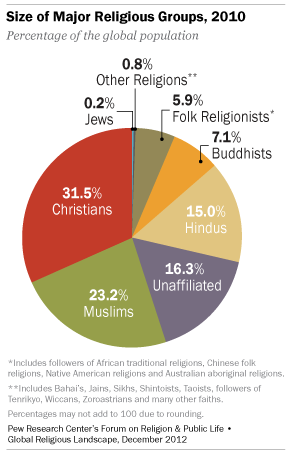

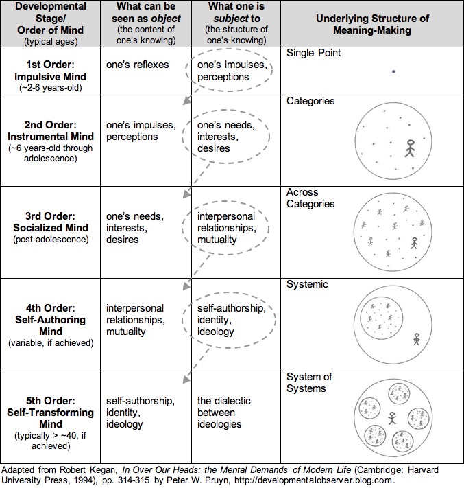


![\[f(x, y) = (x^2 + y - 11)^2 + (x + y^2 - 7)^2\]](https://www.tedtanner.org/wp-content/ql-cache/quicklatex.com-23ec65f33d158fdb3b13461e54d04f1a_l3.png "Rendered by QuickLaTeX.com")
 :
:
 .
.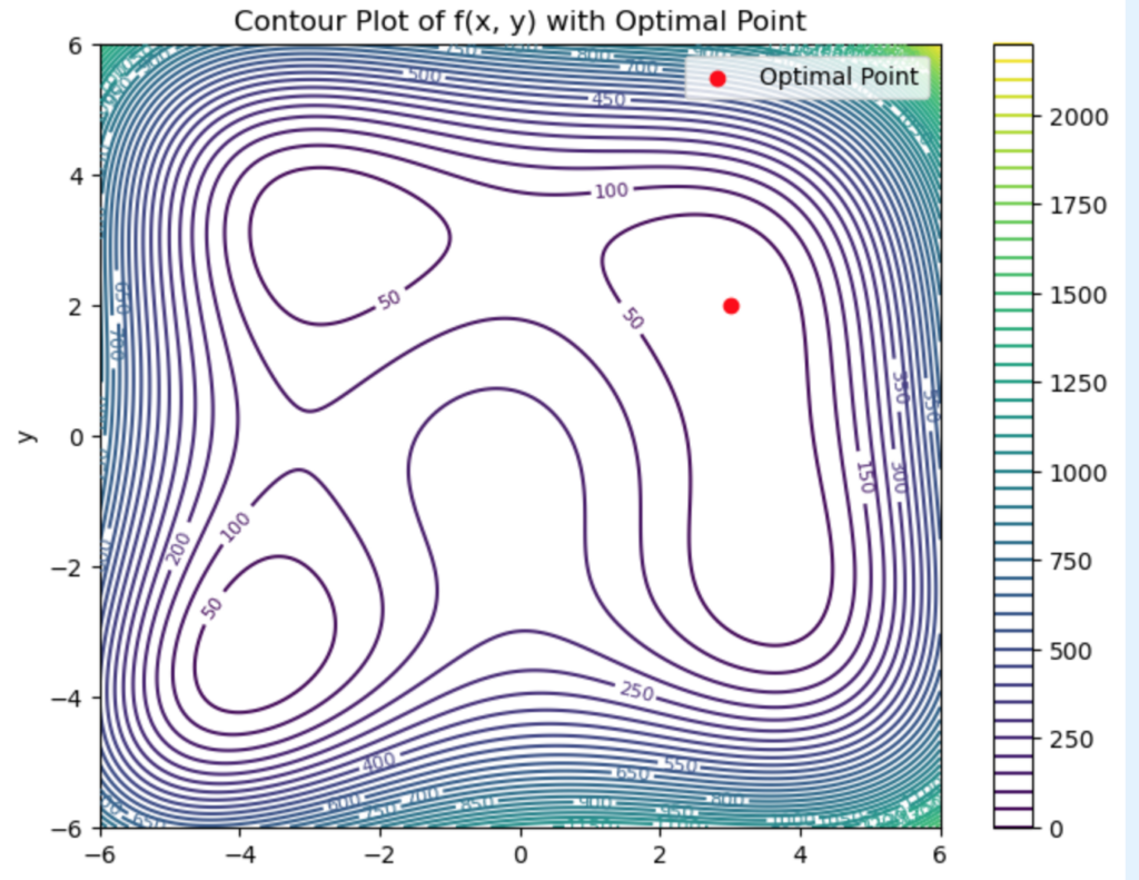
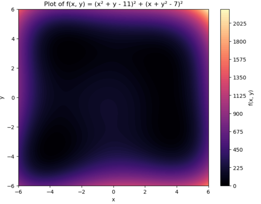
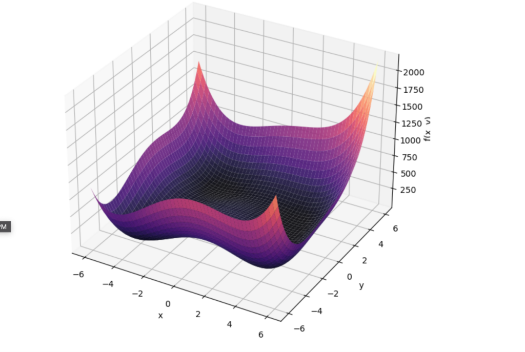

 and a transition matrix
  , where each element
  represents the probability of transitioning from state
  .
.
 , a point in the state space. This point can be chosen randomly or based on prior knowledge.
 , propose a new state
  using a proposal distribution
  , which suggests a candidate for the next state. This proposal distribution can be symmetric (e.g., a normal distribution centered at
  for moving from the current state
 ![\[\alpha = \min \left(1, \frac{\pi(x^) q(x_t | x^)}{\pi(x_t) q(x^* | x_t)} \right)\]](https://www.tedtanner.org/wp-content/ql-cache/quicklatex.com-d0021c453163124b132e82a38dbf20bb_l3.png "Rendered by QuickLaTeX.com")
 , the formula simplifies to:
![\[\alpha = \min \left(1, \frac{\pi(x^*)}{\pi(x_t)} \right)\]](https://www.tedtanner.org/wp-content/ql-cache/quicklatex.com-52d53f2c5d02dc0c354ef060a927b5de_l3.png "Rendered by QuickLaTeX.com")
 from a uniform distribution
 , accept the proposed state
  .
. , reject the proposed state and remain at the current state, i.e.,
  .
. , which changes slowly over time. We’ll use a simple time-series analytics setup to sample this distribution using the Metropolis Algorithm and plot the results. Note: When the target distribution is Gaussian (or close to Gaussian), the algorithm can converge more quickly to the true distribution because of the symmetric smooth nature of the normal distribution.
 ', color='red', linewidth=2)
plt.title("Metropolis Algorithm Sampling with Time-Varying Gaussian Distribution")
plt.xlabel("Time")
plt.ylabel("Sample Value")
plt.legend()
plt.grid(True)
plt.show()
', color='red', linewidth=2)
plt.title("Metropolis Algorithm Sampling with Time-Varying Gaussian Distribution")
plt.xlabel("Time")
plt.ylabel("Sample Value")
plt.legend()
plt.grid(True)
plt.show()
 defines a time-varying mean for the distribution. In this example, it follows a sinusoidal pattern.


 space
space
 𝕋𝕖𝕕 ℂ. 𝕋𝕒𝕟𝕟𝕖𝕣 𝕁𝕣. (@tctjr)
![\[\hat{f} (\xi)=\int_{-\infty}^{\infty}f(x)e^{-2\pi ix\xi}dx\]](https://www.tedtanner.org/wp-content/ql-cache/quicklatex.com-4dfceb039152febfe9d05a834affcd1a_l3.png "Rendered by QuickLaTeX.com")
![\[F(x) &= f\f[k] &= \sum_{j=0}^{N-1} x[j]\left(e^{-2\pi i k/N}\right)^j\0 &\leq k < N\]](https://www.tedtanner.org/wp-content/ql-cache/quicklatex.com-1824d6e88be0eea8520d0874ddd199c6_l3.png "Rendered by QuickLaTeX.com")
![\[f[k] &= f_e[k]+e^{-2\pi i k/N}f_o[k]\f[k+N/2] &= f_e[k]-e^{-2\pi i k/N}f_o[k]\]](https://www.tedtanner.org/wp-content/ql-cache/quicklatex.com-acc567b5572c2d346d8b2f83e18c00a5_l3.png "Rendered by QuickLaTeX.com")
 and
and  which makes it really useful for audio and radar analysis.


![\[x(t)*h(t) &= y(t)\]](https://www.tedtanner.org/wp-content/ql-cache/quicklatex.com-f1aef3d24f6d2ce949b8fc4b8db98b93_l3.png "Rendered by QuickLaTeX.com")
![\[X(f) H(f) &= Y(f)\]](https://www.tedtanner.org/wp-content/ql-cache/quicklatex.com-739e46b1cd83c2130983eef987f18794_l3.png "Rendered by QuickLaTeX.com")
