

Grok 4’s Idea of a Distributed LLM
I was kicking back in my Charleston study this morning, drinking my usual unsweetened tea in a mason jar, the salty breeze slipping through the open window like a whisper from the Charleston Harbor, carrying that familiar tang of low tide “pluff mud” and distant rain. The sun was filtering through the shutters, casting long shadows across my desk littered with old notes on distributed systems engineering, when I dove into this survey on architectures for distributed LLM disaggregation. It’s a dive into the tech that’s pushing LLMs beyond their limits. As i read the numerous papers and assembled commonalities, it hit me how these innovations echo the battles many have fought scaling AI/ML in production, raw, efficient, and unapologetically forward. Here’s the breakdown, with the key papers linked for those ready to dig deeper.
This is essentially the last article in a trilogy. The sister survey is a blog A Survey of Technical Approaches For Distributed AI In Sensor Networks. Then, for a top-level view, i wrote SnakeByte[21]: The Token Arms Race: Architectures Behind Long-Context Foundation Models, so you’ll have all views of a complete system, sensors->distributed compute methods->context engineering.
NOTE: By the time this is published, a whole new set of papers will come out, and i wrote (and read the papers) in a week.
Overview
Distributed serving of LLMs presents significant technical challenges driven by the immense scale of contemporary models, the computational intensity of inference, the autoregressive nature of token generation, and the diverse characteristics of inference requests. Efficiently deploying LLMs across clusters of hardware accelerators (predominantly GPUs and NPUs) necessitates sophisticated system architectures, scheduling algorithms, and resource management techniques to achieve low latency, high throughput, and cost-effectiveness while adhering to Service Level Objectives (SLOs). As you read the LLM survey, think in terms of deployment architectures:
Layered AI System Architecture:
- Sensor Layer: IoT, Cameras, Radar, LIDAR, electro-mag, FLIR etc
- Edge/Fog Layer: Edge Gateways, Inference Accelerators, Fog Nodes
- Cloud Layer: Central AI Model Training, Orchestration Logic, Data Lake
Each layer plays a role in collecting, processing, and managing AI workloads in a distributed system.
Distributed System Architectures and Disaggregation
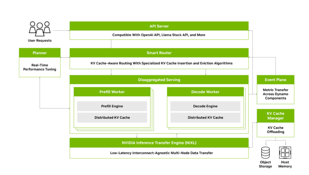
Modern distributed Large Language Models serving platforms are moving beyond monolithic deployments to adopt disaggregated architectures. A common approach involves separating the computationally intensive prompt processing (prefill phase) from the memory-bound token generation (decode phase). This disaggregation addresses the bimodal latency characteristics of these phases, mitigating pipeline bubbles that arise in pipeline-parallel deployments KV-cache Streaming for Fast, Fault-tolerant Generative LLM Serving. As a reminder in LLMs, KV cache stores key and value tensors from previous tokens during inference. In transformer-based models, the attention mechanism computes key (K) and value (V) vectors for each token in the input sequence. Without caching, these would be recalculated for every new token generated, leading to redundant computations and inefficiency.
Systems like Mooncake: A KVCache-centric Disaggregated Architecture for LLM Serving propose a KVCache-centric disaggregated architecture with dedicated clusters for prefill and decoding. This separation allows for specialized resource allocation and scheduling policies tailored to each phase’s demands. Similarly, P/D-Serve: Serving Disaggregated Large Language Model at Scale focuses on serving disaggregated LLMs at scale across tens of thousands of devices, emphasizing fine-grained P/D organization and dynamic ratio adjustments to minimize inner mismatch and improve throughput and Time-to-First-Token (TTFT) SLOs. KVDirect: Distributed Disaggregated LLM Inference explores distributed disaggregated inference by optimizing inter-node KV cache transfer using tensor-centric communication and a pull-based strategy.
Further granularity in disaggregation can involve partitioning the model itself across different devices or even separating attention layers, as explored by Infinite-LLM: Efficient LLM Service for Long Context with DistAttention and Distributed KVCache, which disaggregates attention layers to enable flexible resource scheduling and enhance memory utilization for long contexts. DynaServe: Unified and Elastic Execution for Dynamic Disaggregated LLM Serving unifies and extends both colocated and disaggregated paradigms using a micro-request abstraction, splitting requests into segments for balanced load across unified GPU instances.
The distributed nature also necessitates mechanisms for efficient checkpoint loading and live migration. ServerlessLLM: Low-Latency Serverless Inference for Large Language Models proposes a system for low-latency serverless inference that leverages near-GPU storage for fast multi-tier checkpoint loading and supports efficient live migration of LLM inference states.
Scheduling and Resource Orchestration
Effective scheduling is paramount in distributed LLM serving due to heterogeneous request patterns, varying SLOs, and the autoregressive dependency. Existing systems often suffer from head-of-line blocking and inefficient resource utilization under diverse workloads.
Preemptive scheduling, as implemented in Fast Distributed Inference Serving for Large Language Models, allows for preemption at the granularity of individual output tokens to minimize latency. FastServe employs a novel skip-join Multi-Level Feedback Queue scheduler leveraging input length information. Llumnix: Dynamic Scheduling for Large Language Model Serving introduces dynamic rescheduling across multiple model instances, akin to OS context switching, to improve load balancing, isolation, and prioritize requests with different SLOs via an efficient live migration mechanism.
Prompt scheduling with KV state sharing is a key optimization for workloads with repetitive prefixes. Preble: Efficient Distributed Prompt Scheduling for LLM Serving is a distributed platform explicitly designed for optimizing prompt sharing through a distributed scheduling system that co-optimizes KV state reuse and computation load-balancing using a hierarchical mechanism. MemServe: Context Caching for Disaggregated LLM Serving with Elastic Memory Pool integrates context caching with disaggregated inference, supported by a global scheduler that enhances cache reuse through a global prompt tree-based locality-aware policy. Locality-aware fair scheduling is further explored in Locality-aware Fair Scheduling in LLM Serving, which proposes Deficit Longest Prefix Match (DLPM) and Double Deficit LPM (D2LPM) algorithms for distributed setups to balance fairness, locality, and load-balancing.
Serving multi-SLO requests efficiently requires sophisticated queue management and scheduling. Queue management for slo-oriented large language model serving is a queue management system that handles batch and interactive requests across different models and SLOs using a Request Waiting Time (RWT) Estimator and a global scheduler for orchestration. SLOs-Serve: Optimized Serving of Multi-SLO LLMs optimizes the serving of multi-stage LLM requests with application- and stage-specific SLOs by customizing token allocations using a multi-SLO dynamic programming algorithm. SeaLLM: Service-Aware and Latency-Optimized Resource Sharing for Large Language Model Inference proposes a service-aware and latency-optimized resource sharing framework for large language model inference.
For complex workloads like agentic programs involving multiple LLM calls with dependencies, traditional request-level scheduling is suboptimal. Autellix: An Efficient Serving Engine for LLM Agents as General Programs treats programs as first-class citizens, using program-level context to inform scheduling algorithms that preempt and prioritize LLM calls based on program progress, demonstrating significant throughput improvements for agentic workloads. Parrot: Efficient Serving of LLM-based Applications with Semantic Variable focuses on end-to-end performance for LLM-based applications by introducing the Semantic Variable abstraction to expose application-level knowledge and enable data flow analysis across requests. Conveyor: Efficient Tool-aware LLM Serving with Tool Partial Execution optimizes for tool-aware LLM serving by enabling tool partial execution alongside LLM decoding.
Memory Management and KV Cache Optimizations
The KV cache’s size grows linearly with sequence length and batch size, becoming a major bottleneck for GPU memory and throughput. Distributed serving exacerbates this by requiring efficient management across multiple nodes.
Effective KV cache management involves techniques like dynamic memory allocation, swapping, compression, and sharing. KV-cache Streaming for Fast, Fault-tolerant Generative LLM Serving proposes KV-cache streaming for fast, fault-tolerant serving, addressing GPU memory overprovisioning and recovery times. It utilizes microbatch swapping for efficient GPU memory management. On-Device Language Models: A Comprehensive Review presents techniques for managing persistent KV cache states including tolerance-aware compression, IO-recompute pipelined loading, and optimized chunk lifecycle management.
In distributed environments, sharing and transferring KV cache states efficiently are critical. MemServe introduces MemPool, an elastic memory pool managing distributed memory and KV caches. Infinite-LLM: Efficient LLM Service for Long Context with DistAttention and Distributed KVCache leverages a pooled GPU memory strategy across a cluster. Prefetching KV-cache for LLM Inference with Dynamic Profiling proposes prefetching model weights and KV-cache from off-chip memory to on-chip cache during communication to mitigate memory bottlenecks and communication overhead in distributed settings. KVDirect: Distributed Disaggregated LLM Inference specifically optimizes KV cache transfer using a tensor-centric communication mechanism.
Handling Heterogeneity and Edge/Geo-Distributed Deployment
Serving LLMs cost-effectively often requires utilizing heterogeneous hardware clusters and deploying models closer to users on edge devices or across geo-distributed infrastructure.
Helix: Serving Large Language Models over Heterogeneous GPUs and Networks via Max-Flow addresses serving LLMs over heterogeneous GPUs and networks by formulating inference as a max-flow problem and using MILP for joint model placement and request scheduling optimization. LLM-PQ: Serving LLM on Heterogeneous Clusters with Phase-Aware Partition and Adaptive Quantization supports efficient serving on heterogeneous GPU clusters through adaptive model quantization and phase-aware partition. Efficient LLM Inference via Collaborative Edge Computing leverages collaborative edge computing to partition LLM models and deploy them on distributed devices, formulating device selection and partition as an optimization problem.
Deploying LLMs on edge or geo-distributed devices introduces challenges related to limited resources, unstable networks, and privacy. PerLLM: Personalized Inference Scheduling with Edge-Cloud Collaboration for Diverse LLM Services provides a personalized inference scheduling framework with edge-cloud collaboration for diverse LLM services, optimizing scheduling and resource allocation using a UCB algorithm with constraint satisfaction. Distributed Inference and Fine-tuning of Large Language Models Over The Internet investigates inference and fine-tuning over the internet using geodistributed devices, developing fault-tolerant inference algorithms and load-balancing protocols. MoLink: Distributed and Efficient Serving Framework for Large Models is a distributed serving system designed for heterogeneous and weakly connected consumer-grade GPUs, incorporating techniques for efficient serving under limited network conditions. WiLLM: an Open Framework for LLM Services over Wireless Systems proposes deploying LLMs in core networks for wireless LLM services, introducing a “Tree-Branch-Fruit” network slicing architecture and enhanced slice orchestration.
On the of most recent papers that echo my sentiment from years ago where is i’ve said “Vertically Trained Horizontally Chained” (maybe i should trademark that …) is Small Language Models are the Future of Agentic AI where they lay out the position that specific task LLMs are sufficiently robust, inherently more suitable, and necessarily more economical for many invocations in agentic systems, and are therefore the future of agentic AI. The argumentation is grounded in the current level of capabilities exhibited by these specialized models, the common architectures of agentic systems, and the economy of LM deployment. They further argue that in situations where general-purpose conversational abilities are essential, heterogeneous agentic systems (i.e., agents invoking multiple different models chained horizontally) are the natural choice. They discuss the potential barriers for the adoption of vertically trained LLMs in agentic systems and outline a general LLM-to-specific chained model conversion algorithm.
Other Optimizations and Considerations
Quantization is a standard technique to reduce model size and computational requirements. Atom: Low-bit Quantization for Efficient and Accurate LLM Serving proposes a low-bit quantization method (4-bit weight-activation) to maximize serving throughput by leveraging low-bit operators and reducing memory consumption, achieving significant speedups over FP16 and INT8 with negligible accuracy loss.
Splitting or partitioning models can also facilitate deployment across distributed or heterogeneous resources. SplitLLM: Collaborative Inference of LLMs for Model Placement and Throughput Optimization designs a collaborative inference architecture between a server and clients to enable model placement and throughput optimization. A related concept is Split Learning for fine-tuning, where models are split across cloud, edge, and user devices Hierarchical Split Learning for Large Language Model over Wireless Network. BlockLLM: Multi-tenant Finer-grained Serving for Large Language Models enables multi-tenant finer-grained serving by partitioning models into blocks, allowing component sharing, adaptive assembly, and per-block resource configuration.
Performance and Evaluation Metrics
Evaluating and comparing distributed LLM serving platforms requires appropriate metrics and benchmarks. The CAP Principle for LLM Serving: A Survey of Long-Context Large Language Model Serving suggests a trade-off between serving context length (C), serving accuracy (A), and serving performance (P). Developing realistic workloads and simulation tools is crucial. BurstGPT: A Real-world Workload Dataset to Optimize LLM Serving Systems provides a real-world workload dataset for optimizing LLM serving systems, revealing limitations of current optimizations under realistic conditions. LLMServingSim: A HW/SW Co-Simulation Infrastructure for LLM Inference Serving at Scale is a HW/SW co-simulation infrastructure designed to model dynamic workload variations and heterogeneous processor behaviors efficiently. ScaleLLM: A Resource-Frugal LLM Serving Framework by Optimizing End-to-End Efficiency focuses on a holistic system view to optimize LLM serving in an end-to-end manner, identifying and addressing bottlenecks beyond just LLM inference.
Conclusion
The landscape of distributed LLM serving platforms is rapidly evolving, driven by the need to efficiently and cost-effectively deploy increasingly large and complex models. Key areas of innovation include the adoption of disaggregated architectures, sophisticated scheduling algorithms that account for workload heterogeneity and SLOs, advanced KV cache management techniques, and strategies for leveraging diverse hardware and deployment environments. While significant progress has been made, challenges remain in achieving optimal trade-offs between performance, cost, and quality of service (QOS) across highly dynamic and heterogeneous real-world scenarios.
As the sun set and the neon glow of my screen dimmed, i wrapped this survey up, leaving me pondering the endless horizons of AI/ML scaling like waves crashing on the shore, relentless and full of promise and thinking how incredible it is to be working in these areas where what we have dreamed for decades has come to fruition?
Until Then,
#iwishyouwater
Ted ℂ. Tanner Jr. (@tctjr) / X
MUZAK TO BLOG BY: Vangelis, “L’apocalypse de animax (remastered). Vangelis is famous for “Chariots Of Fire” and “Blade Runner” Soundtracks.

 for each sensor
  .
.![W = [W_{ij}]](https://www.tedtanner.org/wp-content/ql-cache/quicklatex.com-2ce7bdef9ccf58e4ab7e96e648b21a50_l3.png "Rendered by QuickLaTeX.com") based on the network topology, where
based on the network topology, where  if
if  (neighbors including itself), and
  otherwise, with
  for row-stochasticity.
 (up to maximum iterations):
 (local observation measurement, where
  is the observation model and
  is noise).
 (local model update, e.g., Kalman or prediction step).
 with neighbors
  .
. .
.
![\[\text{RoPE}(x_i) = x_i \cos(\theta_i) + x_i^\perp \sin(\theta_i)\]](https://www.tedtanner.org/wp-content/ql-cache/quicklatex.com-ecd25300180f956fe439d5e848c787c0_l3.png "Rendered by QuickLaTeX.com")
 , extended by interpolation.
 . For long sequences, this becomes computationally expensive. Sparse attention addresses this by selectively attending to a subset of tokens, reducing the computational burden. Complexity drops from
  to
to  or better using block or sliding windows.
![\[\text{MoE}(x) = \sum_{i=1}^k g_i(x) \cdot E_i(x)\]](https://www.tedtanner.org/wp-content/ql-cache/quicklatex.com-0192f60a77fdd25f25e0f5f24fdd9e45_l3.png "Rendered by QuickLaTeX.com")

 where
where  and
and  are complex numbers.
 for each point in a grid.
 .
. (iteration values) and output (iteration counts) as zero arrays.
 .
. of a complex number
  .
. (scaled by
  ). For example, y=0.5 y = 0.5 y=0.5 corresponds to a complex number with imaginary part
  .
. , where
  is the x-coordinate (real part) and
  is the y-coordinate (imaginary part).
 ,
, 
 and the Fibonacci sequences (A sequence where each number is the sum of the two preceding ones: 0, 1, 1, 2, 3, 5, 8, 13, 21…) are deeply interconnected through mathematical patterns and structures that appear in nature, art, and geometry. The very essence of our lives.


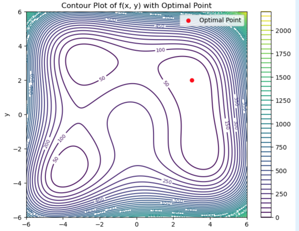
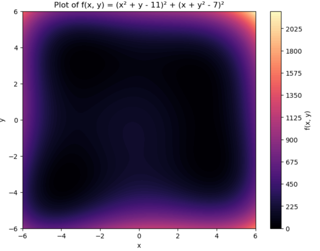
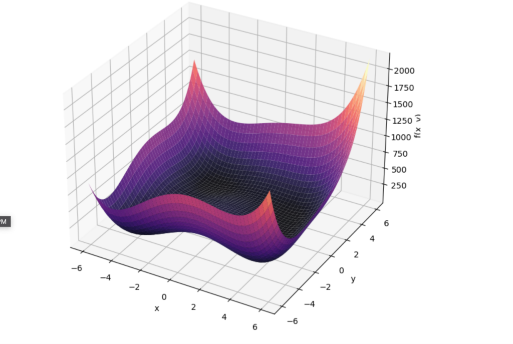
![\[f(x, y) = (x^2 + y - 11)^2 + (x + y^2 - 7)^2\]](https://www.tedtanner.org/wp-content/ql-cache/quicklatex.com-23ec65f33d158fdb3b13461e54d04f1a_l3.png "Rendered by QuickLaTeX.com")
 :
:
 .
.

 and a transition matrix
  , where each element
  represents the probability of transitioning from state
  .
.
 , a point in the state space. This point can be chosen randomly or based on prior knowledge.
 , propose a new state
  using a proposal distribution
  , which suggests a candidate for the next state. This proposal distribution can be symmetric (e.g., a normal distribution centered at
  for moving from the current state
 ![\[\alpha = \min \left(1, \frac{\pi(x^) q(x_t | x^)}{\pi(x_t) q(x^* | x_t)} \right)\]](https://www.tedtanner.org/wp-content/ql-cache/quicklatex.com-d0021c453163124b132e82a38dbf20bb_l3.png "Rendered by QuickLaTeX.com")
 , the formula simplifies to:
![\[\alpha = \min \left(1, \frac{\pi(x^*)}{\pi(x_t)} \right)\]](https://www.tedtanner.org/wp-content/ql-cache/quicklatex.com-52d53f2c5d02dc0c354ef060a927b5de_l3.png "Rendered by QuickLaTeX.com")
 from a uniform distribution
 , accept the proposed state
  .
. , reject the proposed state and remain at the current state, i.e.,
  .
. , which changes slowly over time. We’ll use a simple time-series analytics setup to sample this distribution using the Metropolis Algorithm and plot the results. Note: When the target distribution is Gaussian (or close to Gaussian), the algorithm can converge more quickly to the true distribution because of the symmetric smooth nature of the normal distribution.
 ', color='red', linewidth=2)
plt.title("Metropolis Algorithm Sampling with Time-Varying Gaussian Distribution")
plt.xlabel("Time")
plt.ylabel("Sample Value")
plt.legend()
plt.grid(True)
plt.show()
', color='red', linewidth=2)
plt.title("Metropolis Algorithm Sampling with Time-Varying Gaussian Distribution")
plt.xlabel("Time")
plt.ylabel("Sample Value")
plt.legend()
plt.grid(True)
plt.show()
 defines a time-varying mean for the distribution. In this example, it follows a sinusoidal pattern.


![\[(E_i^*,E_j^*)\]](https://www.tedtanner.org/wp-content/ql-cache/quicklatex.com-4b7772a3028c53b1f55a34079971f64d_l3.png "Rendered by QuickLaTeX.com")
![\[H=-1/N \sum_{i=1}^{N} P_i\,log_2\,P_i\]](https://www.tedtanner.org/wp-content/ql-cache/quicklatex.com-5a3422c3ff70f85af819c83d0790d495_l3.png "Rendered by QuickLaTeX.com")
![\[\frac{\partial u}{\partial t} &= D_u \nabla^2 u + f(u, v),\]](https://www.tedtanner.org/wp-content/ql-cache/quicklatex.com-99147d396c77a8652cc77ac0cab65ffe_l3.png "Rendered by QuickLaTeX.com")
![\[\frac{\partial v}{\partial t} &= D_v \nabla^2 v + g(u, v),\]](https://www.tedtanner.org/wp-content/ql-cache/quicklatex.com-a0acfd5f636e96e9c05ed136c210b906_l3.png "Rendered by QuickLaTeX.com")

![\[\begin{itemize}\item $u$ and $v$ are concentrations of two chemical substances (morphogens),\item $D_u$ and $D_v$ are diffusion coefficients for $u$ and $v$,\item $\nabla^2$ is the Laplacian operator, representing spatial diffusion,\item $f(u, v)$ and $g(u, v)$ are reaction terms representing the interaction between $u$ and $v$.\end{itemize}\]](https://www.tedtanner.org/wp-content/ql-cache/quicklatex.com-3c0fe86ddd76baee1115898f2a4cd86e_l3.png "Rendered by QuickLaTeX.com")

 𝕋𝕖𝕕 ℂ. 𝕋𝕒𝕟𝕟𝕖𝕣 𝕁𝕣. (@tctjr) / X