SnakeByte[23]: Maynard-Cross Learning (MCL): Hive Minds as a Single RL Agent

First i trust everyone is safe.

Second, i have been sitting on a draft SnakeByte for a while about a paper that does what i wish more swarm literature would do. It stops waving its hands at “emergence” and writes the update rule down. Instead of picking a library or method i decided to randomly pick cool papers. i just haven’t had a chance to sit with this one long enough for prime time. This paper caught my eye on the Keywords: Swarm Intelligence, Reinforcement Learning, Evolutionary Game Theory,
Evolutionary Biology.

A population of agents following a simple, local, purely imitative weighted-voter rule is mathematically equivalent to a single abstract reinforcement learning agent that updates its policy with Maynard-Cross Learning.

~ the actual claim

i guess this is where i am supposed to say, “A banger of a paper just dropped, and it shows how you can spin up 1-Billion Agents to make you 1-Billion Dollars In A Month.” i digress.

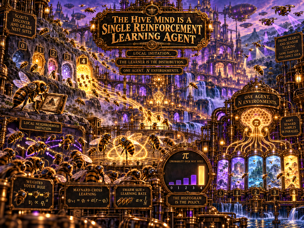
The paper is The Hive Mind is a Single Reinforcement Learning Agent (Soma, Bouteiller, Hamann, Beltrame, arXiv:2410.17517). Honey bees. Nest sites. Waggle dances. The usual natural-history furniture. Underneath that furniture is a bandit. Quantum spooky distance of the hive mind.

Can a single RL Agent perform as The Hive?

What the bees are actually doing

A scout finds a cavity. She grades it the way any field engineer grades a site: volume, exposure, how hard it is to get home. She comes back and dances. Duration and vigor scale with the reward she thinks she sampled. Another bee does not run a comparison. She copies the first dancer she runs into inside a small neighborhood. Blind imitation. Local. Cheap.

Do that with a few hundred scouts and the fraction of the swarm committed to each site starts to behave like a policy . Not a metaphor. A probability vector. The hive is not a mind hovering over the individuals. The hive is the update those individuals implement when you add them up.

MCL is that update. It sits in the same family as Cross Learning, which sits downstream of the replicator story Maynard Smith opened and Taylor, Jonker, Schuster, and Sigmund actually wrote as dynamics. Maynard Smith gave us the equilibrium. Other people wrote the motion. MCL is motion with a normalization the bees accidentally invented.

The discrete rule

One bee, one sample. She is committed to site and comes home with a noisy reward . The population policy moves like this:

   

   

The swarm size is the learning rate. Bigger swarm, smaller step. The organism learns more slowly because there are more of them. That is not a bug. That is averaging. Pretty much the same physics as a learning rate.

You do not know the true mean rewards . So in the denominator is not an oracle. In any implementation that can actually run, is an online estimate. A moving average of rewards already seen. The normalization is “how good was this sample relative to what we have been getting.”

Skip the update when the estimate is sitting on zero. Do not divide by faith.

The continuous limit, and why the extra factor matters

Take the population large and the step small and you land on the Maynard-Smith replicator dynamic:

   

Classic Cross Learning, pushed to the same limit, gives you the Taylor replicator:

   

The only new object is . Absolute rewards wander. Noise wanders with them. Dividing by the current average value keeps the step from blowing up when every site is paying well and from stalling when every site is paying poorly. It is a baseline. Bees did not call it a baseline. The algebra does.

The paper’s conditions for reliable convergence include a neighborhood that is not tiny. Something like before the quorum story gets trustworthy. Local does not mean “talk to one neighbor and call it wisdom.” Local means “small relative to , large enough to estimate a vote.” Hold that sentence. The plots below will test your patience.

One agent, N environments

Read the micro-rule from the macro side and the RL picture snaps into focus.

• Each bee samples an action from . That is her current preference.
• She receives a noisy reward from her own site visit. That is one environment.
• Imitation averages those samples into the next .

That is a single online bandit agent aggregating action-value samples from parallel environments. The individuals are not learners in the gradient sense. They are samplers with a copy rule. The learner is the distribution.

i want to be careful about the evolutionary sentence, because it is the one people will over-claim( omg lets anthropormoisize yet another algorithm). The equivalence supplies a plausible selective pressure for the imitation rule: a group that copies this way is doing group-level reinforcement learning whether or not any bee could tell you that. The paper does not prove that kin selection “favors group-level RL” as a primary result. It shows you a mechanism that would be worth keeping if selection ever got its hands on it. Mechanism first. Story second.

Why i care, and why you might

Most “swarm intelligence” (papers, decks, napkins) still hand you a metaphor and a video of drones in a pretty formation. This hands you a pseudo-compiler. If you know which bandit update you want at the macro scale, you can ask what local imitation rule realizes it. If you already have a local rule, you can ask which RL agent you accidentally built.

That is a design tool. Drone search. Sensor tasking and orchestration. Any flock of cheap agents that should not each be running a policy network. You do not put a sophisticated learner in every airframe. You put a sampler and a dance in every airframe, and you let the population be the learner.

Same mathematics, opposite direction of work. Derive the local rule from the update you want. Or read the update off the rule you already shipped.

The notebook:

# Maynard-Cross Learning: one abstract agent, and the bees it claims to be.
# Soma, Bouteiller, Hamann, Beltrame — arXiv:2410.17517
#
# Macro: streaming MCL. One sample per step. Learning rate alpha = 1/N.
#        v is NOT the true mean reward. It is an exponential moving average
#        of rewards actually observed. That is the version you can ship.
#
# Hive:  N agents. Each holds a discrete site preference.
#        Each step, every agent hears M neighbors and copies with
#        probability proportional to the rewards those neighbors just drew.
#        Nobody stores pi. The histogram of preferences is pi.

import numpy as np
import matplotlib.pyplot as plt

# --- bandit and swarm ---
K = 5            # sites / arms
N = 200          # bees; also sets alpha = 1/N on the macro side
T = 2500         # steps. clocks differ; see the post
delta = 0.15     # uniform noise half-width around each q_a
beta = 0.02      # EMA rate for the online baseline v
M = 8            # neighborhood size for the healthy hive
num_runs = 4     # macro seeds for the mean/std band
SEED = 42

q = np.linspace(0.25, 0.85, K)   # 0.25, 0.40, 0.55, 0.70, 0.85
optimal = int(np.argmax(q))      # arm 4


def run_mcl_macro(T=T, seed=0, q=q):
    """Serial MCL. One environment sample per tick."""
    local = np.random.default_rng(seed)
    alpha = 1.0 / N
    pi = np.ones(K) / K
    v_est = 0.0
    history = np.zeros((T, K))
    arms = np.arange(K)

    for t in range(T):
        history[t] = pi
        k = local.choice(K, p=pi)
        r = np.clip(local.uniform(q[k] - delta, q[k] + delta), 0.0, 1.0)

        # online baseline. first reward seeds it; after that, EMA.
        v_est = r if t == 0 else (1.0 - beta) * v_est + beta * r
        if v_est < 1e-8:
            continue

        # MCL: reinforce k by (1 - pi_k), decay every other arm by pi_a,
        # then scale by alpha * (r / v).
        update = alpha * (r / v_est) * np.where(arms == k, 1.0 - pi, -pi)
        pi = np.clip(pi + update, 0.0, None)
        total = pi.sum()
        pi = pi / total if total > 0.0 else np.ones(K) / K

    return history


def run_hive(T=T, seed=0, M=M, q=q):
    """Explicit bees. No policy vector. Histogram only."""
    local = np.random.default_rng(seed)
    prefs = local.integers(0, K, size=N)   # each bee's current site
    history = np.zeros((T, K))

    for t in range(T):
        counts = np.bincount(prefs, minlength=K).astype(float)
        history[t] = counts / N

        # every bee samples a noisy reward for the site she currently likes
        rewards = np.clip(
            local.uniform(q[prefs] - delta, q[prefs] + delta), 0.0, 1.0
        )

        # one neighborhood draw per bee, then a weighted copy
        new_prefs = prefs.copy()
        neigh = local.integers(0, N, size=(N, M))
        for i in range(N):
            js = neigh[i]
            votes = np.bincount(prefs[js], weights=rewards[js], minlength=K)
            total = votes.sum()
            if total > 0.0:
                new_prefs[i] = local.choice(K, p=votes / total)
        prefs = new_prefs

    return history


pi_macro = run_mcl_macro(seed=SEED)
pi_hive = run_hive(seed=SEED, M=8)
pi_hive_small = run_hive(seed=SEED, M=2)   # thin vote; easy bandit still locks

percent_opt = np.vstack([
    run_mcl_macro(seed=SEED + r)[:, optimal] * 100.0
    for r in range(num_runs)
])
mean_opt = percent_opt.mean(axis=0)
std_opt = percent_opt.std(axis=0)

# Figure 1 — full policy, both ontologies
fig, axes = plt.subplots(1, 2, figsize=(12, 5), sharey=True)
for a in range(K):
    axes[0].plot(pi_macro[:, a], label=f"arm {a}  q={q[a]:.2f}")
    axes[1].plot(pi_hive[:, a], label=f"arm {a}  q={q[a]:.2f}")
axes[0].set_title("Macro MCL (one abstract agent)")
axes[1].set_title(f"Hive (N={N} bees, neighborhood M={M})")
for ax in axes:
    ax.set_xlabel("step")
    ax.set_ylabel(r"policy mass ")
    ax.set_ylim(0, 1.02)
    ax.grid(True, alpha=0.3)
    ax.legend(fontsize=8, loc="center right")
fig.tight_layout()
fig.savefig("mcl_policy_evolution.png", dpi=140)

# Figure 2 — mass on the best arm, plus a too-easy small neighborhood
fig, ax = plt.subplots(figsize=(12, 5.5))
ax.plot(pi_macro[:, optimal] * 100.0, color="C0", lw=2.0, label="Macro MCL (this seed)")
ax.plot(pi_hive[:, optimal] * 100.0, color="C1", lw=2.0, label="Hive, M=8")
ax.plot(pi_hive_small[:, optimal] * 100.0, color="C3", lw=1.6, label="Hive, M=2 (too local)")
ax.plot(mean_opt, color="black", lw=1.4, ls="--", label=f"Macro mean over {num_runs} seeds")
ax.fill_between(
    np.arange(T), mean_opt - std_opt, mean_opt + std_opt,
    color="0.2", alpha=0.15, label="macro +/- 1 std",
)
ax.set_xlabel("step")
ax.set_ylabel("percent of mass on the best arm")
ax.set_title("Same bandit, three stories: abstract update, healthy hive, thin vote")
ax.set_ylim(0, 105)
ax.grid(True, alpha=0.3)
ax.legend(loc="center right", fontsize=9)
fig.tight_layout()
fig.savefig("mcl_optimal_convergence.png", dpi=140)
plt.show()

print(f"final macro   {pi_macro[-1, optimal]:.3f}")
print(f"final hive M8 {pi_hive[-1, optimal]:.3f}")
print(f"final hive M2 {pi_hive_small[-1, optimal]:.3f}")

Ok what is all of this doing?

On this seed the final mass on the best arm is 0.952 for the abstract MCL agent, 1.000 for the hive with (M=8), and 1.000 for the hive with (M=2).

That is exactly what the plots show. The abstract agent converges steadily. The hive converges “violently”. (Ya know you have to have some human adjective for code or a storm).

If your hive runs slower, change the problem before you change the theory. Shrink the reward gap. Increase the noise. Make the vote harder. That is the next experiment. If the macro agent converges toward the best arm and the hive does not under the same reward structure, then look at the voting implementation first. The equivalence is not rescued or refuted by a bad bincount.

A batch macro update would give you the fairer clock: draw actions from , collect rewards, average the MCL increments, and apply the aggregate update once. At that point the blue macro curve should stop looking quite so lazy.

Note your probably wondering why not use DEAP? It is the wrong first tool. Nothing here is evolving a genome or code base. This is a probability distribution concentrating under reinforcement. If, later, you want to evolve the dance itself so that a local swarm rule realizes some other desired macro-level bandit update, then put run_hive inside a fitness function and evolve the microscopic rule. Different experiment. Different blog. Maybe sometime in the future.

This one is the equivalence, watched with the lights on cause i’d rather see bees than hear them.

What the run actually did

Five arms. Mean rewards:

   

Uniform reward noise has half-width

   

with samples clipped to ([0,1]).

Arm 4 is optimal with expected reward (q_4=0.85).

The swarm contains

   

bees, which also sets the serial macro learning rate to

   

The online value baseline uses an exponential moving average with

   

The run lasts (T=2500) steps. The healthy hive uses a neighborhood size (M=8). A second hive uses (M=2). We repeat the macro comparison across four seeds.

Same bandit. Same reward noise. Same initial ignorance. Very different clocks.

Figure 1 — Macro MCL policy evolution

The abstract MCL agent begins uniformly:

   

for all five arms.

From there, arm 4 starts accumulating mass while the weaker alternatives are progressively starved.

The movement is not monotonic because the agent is sampling noisy rewards one observation at a time. Arm 3, with (q=0.70), survives longest because it is the nearest competitor. The lower-reward arms disappear much earlier.

For the seed shown:

• around step 100, arm 4 holds (0.213) of the policy;
• around step 500, it holds (0.518);
• around step 1000, it holds (0.725);
• at step 2499, it holds (0.952).

Across the four macro seeds, the final mass on arm 4 ranges from approximately (91.5%) to (97.9%), with a final mean of (95.2%) and a standard deviation of about (2.37) percentage points.

The walk is noisy. The destination is not (which is usually always the case in life).

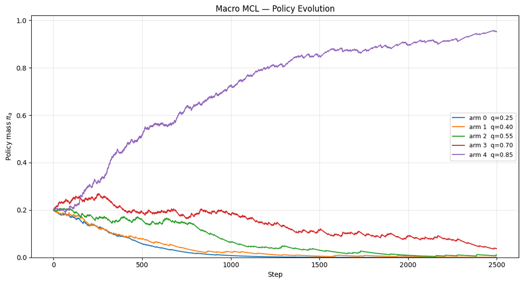
Figure 2 — Hive policy evolution, (M=8)

The hive is doing something operationally very different. This is a test of the public bee broadcasting system this is only a test.

There is no global stored anywhere. Will we converge? The suspense is killing me i hope it lasts!

Each bee carries only a discrete site preference. Each bee samples a noisy reward from that site. Each bee then looks at (M=8) randomly selected neighbors and copies a site according to the neighbors’ reward-weighted votes. The policy exists only as the histogram of those preferences. And that histogram locks fast.

With (N=200) and (M=8), the optimal arm exceeds (95%) of the population by about step 22, exceeds (99%) by about step 24, and reaches complete fixation by about step 33.

The other four traces collapse onto the floor. That does not mean the hive discovered a better learning rule. It means the hive is consuming much more information per tick (i’m not sure if that is the correct wording; you can’t consume information?). The serial macro loop samples one action and one reward per step.

The hive samples roughly (N=200) rewards and performs roughly (N=200) local imitation decisions per step. Same family of mathematics. Very different amount of work per tick.

That distinction matters.

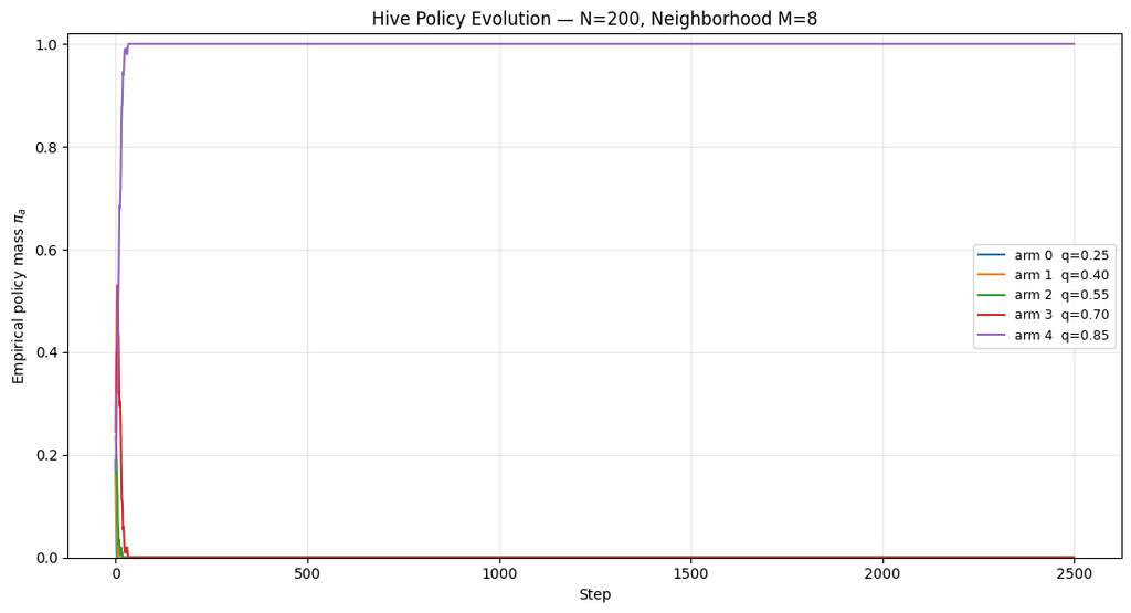
Figure 3 — Best-arm convergence

The convergence plot makes the clock mismatch explicit.

• Blue is the serial Macro MCL run for seed 42.
• Orange is the hive with (M=8).
• Green is the hive with (M=2).
• The dashed red line is the mean of the four macro runs.
• The shaded band is standard deviation across those macro runs.

Both hive variants race to the ceiling while the macro agent climbs gradually toward the same winner.

The (M=8) hive reaches complete fixation at roughly step 33.

The (M=2) hive takes longer, but only slightly: it exceeds (95%) around step 37 and reaches complete fixation around step 58.

So on this particular bandit, (M=2) does not fail.

That is important.

The reward means are spaced by (0.15), and the noise half-width is also (0.15). Arm 4 is sufficiently better than the alternatives that even a very thin neighborhood vote usually discovers the correct direction.

The paper’s warning about very small neighborhoods concerns reliability when the alternatives are harder to distinguish: smaller reward gaps, heavier noise, or situations where a lucky local sample can pull a tiny neighborhood into premature consensus. That is the experiment to run next. Let’s Shrink the gap.

Now let us increase .

Then see whether (M=2) starts believing the first charismatic (tiny) dancer it meets. Hold me close. Get the lyric?

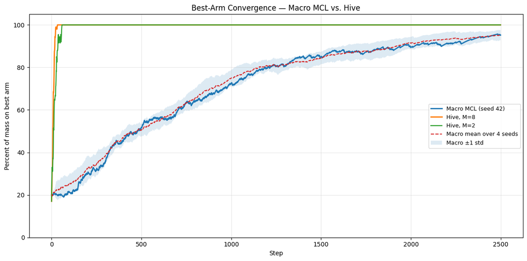
Figure 4 — Early-time convergence

The early-time zoom is probably the clearest picture in the set because it removes the long flat tail after the hive has already converged. Within the first 250 steps, the distinction is obvious.

The (M=8) hive climbs from roughly (20%) initial representation to complete fixation in only a few dozen collective updates.

The (M=2) hive is somewhat noisier and slower, but still reaches fixation before step 60.

Over the same interval, the serial macro agent is still wandering between roughly (20%) and (30%) policy mass on the optimal arm.

Again: do not read that as intelligence. Read the clock. One side is processing one reward sample per tick. The other side is processing a population-sized batch. The comparison is deliberately unfair in wall-clock information because that unfairness exposes the architecture.

If you want schedule equivalence, batch the macro learner with (B=N), or slow the hive down to one imitation event per tick. What the plots show cleanly is something narrower and more interesting: the abstract update and the swarm of local copiers select the same arm. They agree on the destination. They do not agree on the schedule. The destination is the mathematical equivalence. The schedule is an implementation choice.

Confusing those two is like looking at the orange line, looking at the blue line, and deciding the theorem must be wrong because one of them has a faster clock.

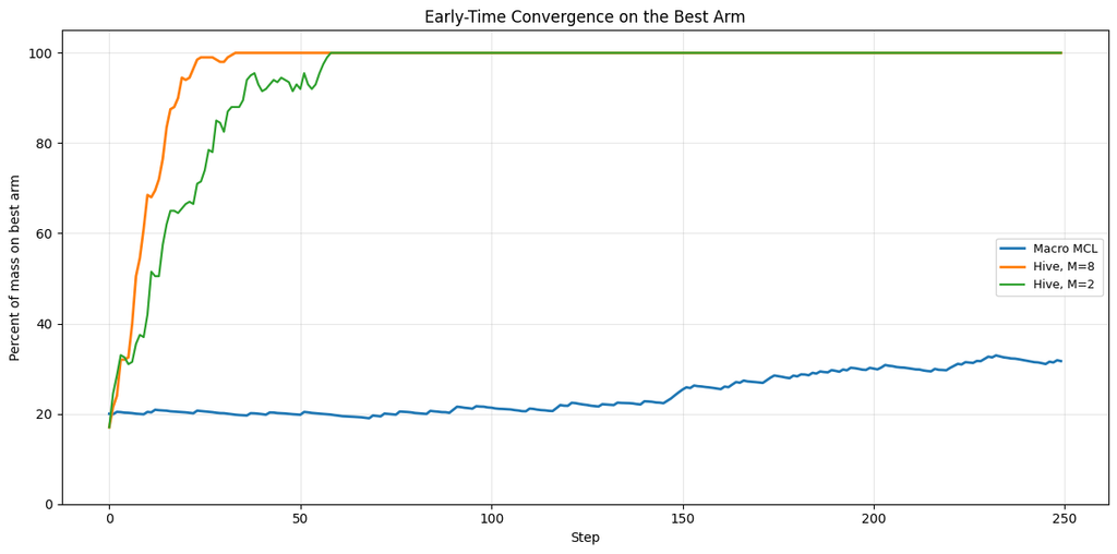
The early-convergence zoom is particularly useful because it makes the clock mismatch visually obvious: the hive gets essentially to 100% within tens of collective updates while serial MCL is still around 20–30%. That directly illustrates the explanation that the “macro loop” consumes one reward per tick while the hive is consuming roughly fresh observations per collective tick

Broader Implications For Maynard Learning

A swarm of cheap physical agents does not need a genius in every airframe. The paper’s equivalence says the opposite: if each body only samples and imitates locally, the population itself is already one online learner, aggregating noisy rewards across many parallel environments. In defense tech and physical AI that is a design rule, not a metaphor. A flock of scouts, buoys, or small unmanned vehicles can search, sense, and commit to a site, a route, or a task by a weighted-voter dance whose macro-update is Maynard-Cross Learning, with learning rate set by how many bodies you field and with no central policy server in the loop. Individuals stay simple, sometimes even “irrational” if you grade them one at a time. The group still converges. You get scale, you lose the single radio that everyone is waiting on, and you design the local copy rule so the hive you actually built is the bandit agent you meant to field.

It challenges traditional views of “intelligence” (the stochastic parrots will tell you they are) as individual-centric, showing how distributed systems can rival advanced RL agents through emergence.

Until Then,

#iwishyouwater <- the swarm does not have a leader. West Palm Beach Doing THE THANG.

#EverForward, stay local and still converge.

𝕋𝕖𝕕 ℂ. 𝕋𝕒𝕟𝕟𝕖𝕣 𝕁𝕣. (@tctjr) / X

MUZAK TO BLOG BY: Madman Across The Water, Tiny Dancer. Of course, Bernie Taupin was a lyrical genius, and well, you go play and sing like the madman – hold me closer, Tiny Dancer. Then i thought maybe Choo Choo Cha Choo? I am he, As you are he, As you are me, And we are all together, convergence if you will. The Oingo Boingo version is fire. Then again there is no one like the original.

Footnotes

[1] John Maynard Smith founded the ESS idea. The continuous replicator equation came later (Taylor & Jonker; Schuster & Sigmund). ESS is what the dynamics often sit down on. Do not hand him the differential equation. He already has enough credit. John Maynard Smith is also recognized as the founder of evolutionary game theory, providing the essential framework and the ESS concept that underpins the field, which later researchers, including those who formulated replicator dynamics, built upon. While Maynard Smith’s initial work focused on the static equilibrium concept of ESS, the replicator dynamics is a related concept developed later by other researchers (notably Taylor and Jonker, and Schuster and Sigmund) to describe the process of how strategies change in a population over time. The replicator equation is a set of differential equations that models how the frequency of a given strategy increases if its payoff (fitness) is higher than the average payoff of the population. The ESS is the stable, stationary point that the replicator dynamics often converge to. 

[2] Cross Learning is the “imitation of success” aggregate. MCL is the weighted-voter aggregate. Same family, different micro-rule, different in the limit. If you implement CL by deleting the division, you can watch the robustness claim instead of taking my word for it.

[3] IS IT still ok to use jupyter notebooks? Is it like bell bottoms that might come back into vogue one day?

[4] Is it straight edge or punk to write your own LATEX?

[5] Hat tip to Fiona Cashin, keep those bees healthy. Great talking to you.