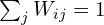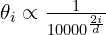
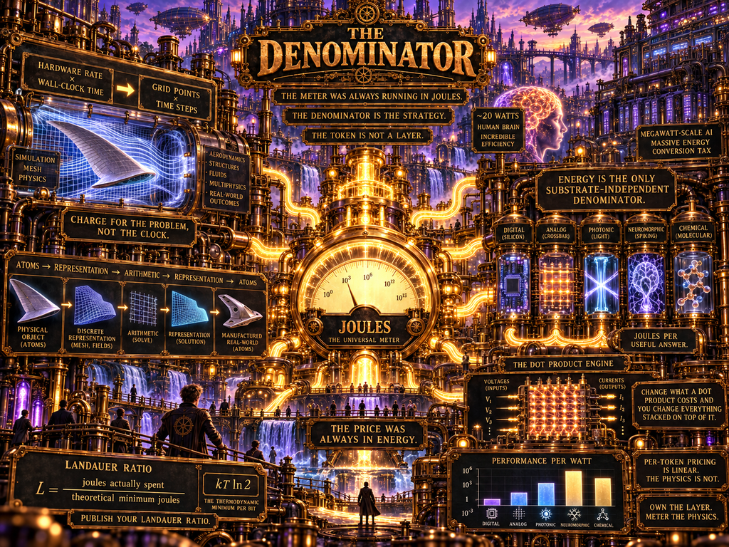
Distributed_Computing | Theodore C. Tanner Jr.

The Denominator (aka The Meter Was Always Running In Joules)

“Information is not a disembodied abstract entity; it is always tied to a physical representation.”
Rolf Landauer, The Physical Nature of Information, Physics Letters A 217 (1996), 188–193

First, i trust everyone is safe.

Second, this one starts with a pricing page, which is an unpromising place to begin an essay about physics. Stay with me. What looks like a billing decision turns out to be a physics argument wearing a costume.

The company is Flexcompute³. They sell simulation computational fluid dynamics, and finite-difference time-domain electromagnetics, two workloads that have been eating supercomputers alive for as long as there have been supercomputers to eat. And they do not charge you for the computer.

They charge you for the problem.

The Word Itself

i always start with the word, Dear Reader, because the word usually knows more than the pitch deck.

Credit, from the Latin credere. To believe. To entrust. A credit is a belief about value held between two parties, and it is worth exactly what the issuing party says it is worth, right up until the moment they say otherwise. Every loyalty point, every arcade token, every airline mile, every cloud dollar. A belief.

Joule, from James Prescott Joule, who spent years measuring the mechanical equivalent of heat by churning water with a paddle wheel and watching the temperature rise. A joule is not a belief. Nobody can reprice it. It is a kilogram-meter-squared per second-squared and it will be that in Charleston, in Reston, on the moon, and after every company in this essay is a footnote.

Denominator, from denominare. To name. The thing that does the naming.

Hold those three. The whole essay is in there.

What They Actually Did

Here is the legacy model, which is the model essentially every cloud has used since the day cloud became a word:

$\text{Cost} \;=\; \text{Hardware Rate} \times \text{Wall-Clock Time}$

Innocent-looking. It is not innocent. Sit with it for a second and you will see the problem, and once you see it you cannot unsee it anywhere in this industry.

If i bill you by the hour, i get paid more when my software is worse.

That is not a cynical reading. That is the arithmetic. A badly optimized solver running on a stalled node behind a queue is, to the provider, indistinguishable from a good quarter. The incentive gradient points directly away from the thing the customer wants. Everyone in the chain knows this and everyone has agreed not to mention it, the way you do not mention that the bar is pouring doubles.

Flexcompute changed the denominator. Their currency, the FlexCredit, is computed like this:

$\text{FlexCredits} \;\propto\; N_{\text{grid}} \times N_{\text{steps}}$

Spatial resolution times temporal resolution. The Tidy3D documentation says it plainly: a FlexCredit reflects the size of a simulation, in both grid points and timesteps, and it explicitly does not reflect the compute time required to run it⁴. (i am scoping that to Tidy3D on purpose, because that is the FAQ i read. Confirm the Flow360 terms separately before quoting them⁵ a company can run different billing models on different solvers, and i am not going to assume one from the other.) When you upload a job the system prints the maximum cost before a single cycle burns. If the physics converge early and the solver shuts off, the bill is prorated down⁶.

Read what that does to the incentive.

Now if their solver is slow, they tie up their own silicon longer and earn exactly the same number of credits. The risk moved across the table. They are now structurally obligated to write the fastest code on earth, because every hour they shave is an hour of their own hardware they get back. Their own documentation offers a rough benchmark: one FlexCredit is somewhere around fifty hours of traditional CPU core time for FDTD⁷. Their job is to make that number keep falling, and the pricing model is what makes it their job.

Plenty of companies write mission statements about customer alignment. This is one of the few that put it in the arithmetic instead, where it cannot be walked back by a new VP.

#TCTRules: The denominator is the strategy. Everything above it is marketing.

And Now On With The Show

Because grid points times time steps is a good denominator. It is not the last one.

It is a model of the work. A very good model – it is the literal mathematical definition of the problem, which is why it feels so clean. But it is still a human-chosen proxy that a company issues and a company could, in principle, reprice. It is a credit. It is a belief.

Go one level down and you hit the thing nobody issues.

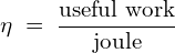
$\eta \;=\; \frac{\text{useful work}}{\text{joule}}$

Normalized compute per unit of power. FLOPS per watt, tokens per joule, useful answers per kilowatt-hour. The Green500 has ranked supercomputers this way for years⁸, which tells you the people closest to the metal worked this out a long time ago while the people writing the invoices did not.

And here is why it is a different kind of number than everything above it.

Hours drift. A 2015 hour and a 2026 hour buy wildly different amounts of computation, which means every contract denominated in hours is silently repriced by Moore’s law and nobody renegotiates. Instance types drift the same label buys different silicon in different regions in different years. Seats drift. Credits drift, because the issuer can change the conversion.

A joule is defined by physics, not by a vendor. It is the one quantity in the entire stack anchored to the universe instead of to a price list.

Be careful with that sentence, though, because a joule drifts too just not where you expect. It drifts in two places, and neither of them is the definition.

It drifts in price. Electricity costs wildly different amounts in different places and at different hours several fold, routinely, between a Virginia afternoon and an Icelandic midnight.

It drifts in what it buys. The number of computations a joule pays for has roughly doubled every year and a half for most of the field’s history, slowing to about every two and a half years since 2000⁸. A 2015 joule and a 2026 joule buy wildly different amounts of computation, exactly as the hours do. That is the eight or nine orders of headroom from the next section, being spent in real time.

So the joule is not immune to drift. What it does is put the drift where you can see it. An hour folds efficiency, silicon, and margin into one opaque rate, and the vendor’s internal business stays internal. A joule splits the same drift into two public numbers: a price you can index and hedge, and an efficiency – useful work per joule – you can measure. The thing that does not drift is the problem itself: a converged simulation, a retained token, a validated answer. Price that against a reference joule count that is revised on a published schedule, and the drift stops being hidden and starts being shared. That is the whole proposal, and i will get to it.

The Floor

Now go all the way down, because this is where it stops being an economics essay and becomes a physics one.

There is a hard thermodynamic bottom to computation and we have known about it since 1961⁹. Landauer’s principle: erasing one bit of information dissipates at least $k_{B}T\ln 2$ of energy as heat. Run the numbers at room temperature, 300 kelvin:

$E_{\min} \;=\; k_{B}T\ln 2 \;\approx\; 2.87 \times 10^{-21}\ \text{J}\quad (T = 300\ \text{K})$

Two point eight seven zeptojoules¹⁰. Which means one joule, spent perfectly, with no waste whatsoever, buys you about $3.5 \times 10^{20}$ bit erasures. That is the floor. Not an engineering target – a floor, the way the speed of light is a floor.

The honest footnote, because the physics in this blog is not allowed to be knowingly false: the bound is on erasure, not on computation as such. Reversible computation can in principle dodge it¹¹, which is a genuinely open and genuinely interesting corner of the field. But every machine any of us has ever shipped erases constantly, and every one of them is running something like eight or nine orders of magnitude above that floor.

Eight or nine orders of magnitude. Sit with that. We are not near the wall. We are not even in the same county as the wall. Everything between here and there is headroom, and headroom is where value lives.

And Shannon got there before Landauer did, from the other direction. The Shannon limit says there is a minimum energy per bit for reliable communication: $E_b/N_0$ cannot go below $\ln 2$ , which is -1.59 dB¹². Information theory and thermodynamics, walking into the same bar from opposite doors, and both of them ordering in joules.

The price was always in energy. We have simply been billing in a proxy currency and calling the proxy the thing.

The Token Is Not A Layer

“The choice of a logarithmic base corresponds to the choice of a unit for measuring information.”
Claude E. Shannon, A Mathematical Theory of Communication, Bell System Technical Journal 27 (1948), 379–423

Dirt To First Token through the energy layer.

Owning a layer and choosing a denominator are two different moves. The layer is the thing you own, and other people stand on. The denominator is the unit you meter it in. You can own a layer and meter it stupidly. You can pick a brilliant denominator for a layer you don’t own; that is called being a reseller.

Which brings me to the token, and i want to say this plainly because a lot of money is currently confused about it:

A token is not a layer. A token is a unit of account.¹³

Nobody owns tokens. They are the metering unit for a layer that somebody else owns: silicon, memory bandwidth, and a power purchase agreement. Confusing the two is how a company ends up believing its moat is a billing unit.

And here is the part that should make every person reading this sit up, because the token denominator has the same bug the hour has, just rotated.

Per-token pricing is linear. The physics is not.

i wrote about this in SnakeByte[21]¹⁴, about the long-context arms race: standard self-attention has computational complexity that scales quadratically with the sequence length $\bigl(\mathcal{O}(n^{2})\bigr)$ ¹⁵. So a hundred thousand token prompt is not a hundred times a one thousand token prompt at the attention step. It is far worse than that. The invoice says linear. The silicon says quadratic.

Any time the price curve and the cost curve have different exponents, somebody is eating the difference, and the pressure that creates does not point at making long context genuinely cheap. It points at quietly capping the window, degrading retrieval, truncating the middle, and hoping nobody runs the experiment. Same adversarial gradient as the hour. Different rotation.

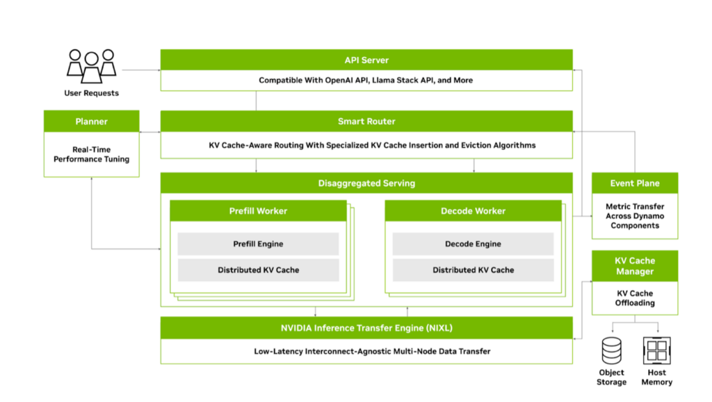
It gets worse, and better, when you look at what is physically happening. Prefill processing the prompt is compute-bound. Decoding, generating the next token, is memory-bound. i surveyed this at length in the disaggregation piece¹⁶ and the whole reason the field is splitting those phases onto separate clusters is that they are two different machines pretending to be one.

Two different machines means two different energy profiles. Moving a byte out of high-bandwidth memory costs substantially more energy than doing arithmetic on it once it has arrived¹⁷.

Providers do not charge one flat rate per token. They already tier. Output tokens run roughly three to six times the price of input tokens the median across the market sits near four and cached input is routinely discounted to something like a tenth of a fresh input token. Some models have started charging a long-context surcharge above a couple of hundred thousand tokens¹⁸.

Look at what that tiering actually is. Input is prefill, which is compute-bound. Output is decode, which is memory-bound. Cached input is prefill you already paid for and do not have to redo. The pricing sheet has been quietly converging on the physics for two years and nobody has said so out loud. It is the same move Flexcompute made, arrived at by trial and error instead of by design.

Which makes the remaining gap the interesting part, and it is still a gap. Three buckets is not a measurement. Input, output and cached is a coarse quantization of a continuous cost surface, set by what the market will bear and revised when margins hurt – and inside every one of those buckets the exponent mismatch is still running, because attention is quadratic and the bucket is priced per token. The surcharge above two hundred thousand tokens is the tell. That is not a pricing strategy. That is a quadratic poking through a linear schedule hard enough that somebody had to patch it.

i already proposed a better denominator without quite noticing i had. In that same piece i suggested metered billing based on tokens stored and tokens retrieved – which separates the memory term from the compute term, and is therefore closer to the physics than a flat per-token rate. That is exactly the move Flexcompute made. Split the proxy into the parts that actually cost different amounts.

And one level below mine is the one i did not write, which is this whole essay:

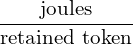
$\frac{\text{joules}}{\text{retained token}}$

i ended that post with the architectural arms race is becoming a memory computation problem, and then i signed off with Got More Ram? i meant it as a joke about capacity.

It is not a capacity question. Memory movement is where the energy goes. Got more ram is an energy question wearing a capacity costume, and i did not see it until i went looking for the denominator underneath my own denominator.

Atoms, Bits, Atoms

Here is why physics-based simulation is the right place to have found this argument, and not an accident that it showed up there first.

Simulation is a round trip. It starts in atoms and it ends in atoms, and everything in between is a detour through representation.

$\text{atoms} \;\rightarrow\; \text{representation} \;\rightarrow\; \text{arithmetic} \;\rightarrow\; \text{representation} \;\rightarrow\; \text{atoms}$

A wing exists. Air exists. Neither of them is doing math. The air is simply obeying Navier-Stokes because it has no choice, in continuous time, at no computational cost to itself, everywhere at once. We cannot watch that directly at the resolution we need, so we chop the wing into a mesh, chop time into steps, quantize every continuous quantity into a finite number of bits, and then ask a machine to imitate what the air was already doing for free.

Then we convert back. We cut metal. We etch a photonic circuit. Atoms again.

Every one of those arrows is a conversion, and every conversion is a tax paid in energy and fidelity. This is the same border i wrote about in the analog essay¹⁹, with the stakes raised: life is not band-limited, and neither is a wing in turbulent flow. We sample it anyway because countability is a magnificent trade. But we should at least know what we are being charged.

And look at what the arithmetic in the middle actually is. Strip away the frameworks and the schedulers and the driver stack and you reach the same irreducible operation in almost every workload that matters right now:

The Almighty Dot Product.

Multiply a row by a column and accumulate. That is a CFD (computational fluid dynamics) solver doing a sparse matrix-vector product inside a Krylov iteration. That is a finite element code applying a stiffness matrix. That is attention computing how much one token cares about another. That is a convolution. The GPU won the last decade not because it is a graphics device but because it is a dot product device, and the whole industry quietly reorganized itself around the one primitive the hardware does well.

For anybody who has not spent a career inside a solver: CFD is simulating how a fluid moves. Air over a wing. Water through a pump. Blood through an artery. FEA is finite element analysis, simulating how a solid deforms and where it fails. The load on a bracket, the stress in a bridge, a phone chassis meeting a sidewalk. Even acoustical rendering. All work the same way: chop the thing into millions of small pieces, write down how each piece affects the pieces touching it, and solve. That stiffness matrix K is exactly that bookkeeping for a structure – how every piece pushes back on every other piece.

For those that remember it, here is the math. One operation:

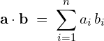
$\mathbf{a}\cdot\mathbf{b} \;=\; \sum_{i=1}^{n} a_{i}\,b_{i}$

And here is that same operation wearing four different hats:

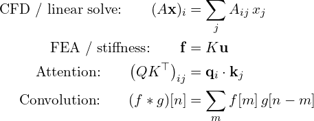
$\begin{aligned} \text{CFD / linear solve:}\qquad (A\mathbf{x})_{i} &= \sum_{j} A_{ij}\,x_{j} \\ \text{FEA / stiffness:}\qquad \mathbf{f} &= K\mathbf{u} \\ \text{Attention:}\qquad \bigl(QK^{\top}\bigr)_{ij} &= \mathbf{q}_{i}\cdot\mathbf{k}_{j} \\ \text{Convolution:}\qquad (f * g)[n] &= \sum_{m} f[m]\,g[n-m] \end{aligned}$

Four fields, four vocabularies, four sets of conferences that do not talk to each other. One sum of products.

And i want to make the strong version of that claim, because it is the point and not a footnote. These are not four analogous operations. They are the same operation. Each one is a bilinear form – a sum of products – and every one of them can be written as

$\mathbf{y} \;=\; M\mathbf{x}$

for some matrix $M$ . The only thing that changes between the four is what $M$ looks like. Sparse for CFD and FEA, because a cell or an element only touches the ones next to it. Toeplitz for convolution, because the same kernel slides along the signal and every row is the row above it shifted by one. Dense for attention – and this is the genuinely new thing in the list – with the matrix produced by the data at runtime rather than fixed in advance by the geometry of a wing or a bracket.

What belongs to this family is the $QK^{\top}$ kernel and the final multiplication by $V$ . The softmax sitting between them is not a bilinear form and is not the same operation at all. Attention is a sandwich of two dot-product layers with a nonlinearity in the middle. The bread is the same. The filling is not.

Same function. Different structure. And here is why that matters for an essay about energy: the structure is where the joules hide. A sparse matrix, a sliding kernel, and a dense data-dependent matrix have wildly different memory access patterns, and memory movement is what costs. The arithmetic is identical across all four. The energy is not even close. Which is exactly the gap a denominator ought to be measuring and the hour never could.

Underneath all of it is the single instruction the silicon actually executes – multiply, add it to what you already had, keep going:

$c \;\leftarrow\; c + a\,b$

That is the whole machine. Everything else is scheduling.

Which means the leverage point is not the model and it is not the framework. Change what a dot product costs and you change everything stacked on top of it, all the way up to the invoice.

Now the part that made me want to write this section.

In a digital machine, a multiply-accumulate is hundreds to thousands of transistors switching, each one dragging charge across a capacitance and dumping it into the heat sink. In an analog crossbar, you apply voltages along the rows, store the weights as conductances at the crosspoints, and let Ohm’s law do the multiply and Kirchhoff’s current law do the sum. The answer arrives on the wire as a current. One step. No clock. No instruction fetch²⁰.

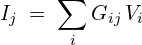
$I_{j} \;=\; \sum_{i} G_{ij}\,V_{i}$

Look at that sum, then look back at the dot product. Same equation. Conductance standing in for one operand, voltage for the other, and Kirchhoff performing the accumulation for free, because current arriving at a node has nowhere else to go.

Read the symbols slowly, because each one is doing something a digital machine has to work for.

$G_{ij}$ is conductance – the reciprocal of resistance, measured in siemens, which is a unit named after a man and not a committee. $V_i$ is the voltage you put on row $i$ . And Ohm’s law, written in the conductance form, says the current through that crosspoint is $G_{ij}V_i$ .

The multiplication happens because the device exists. Nobody issued an instruction. There is no opcode for it. Apply a voltage to a resistor and the multiplication has already occurred by the time you finish reading this sentence, because the electrons are not waiting for a clock edge.

Then the sum. Every crosspoint on column $j$ dumps its current onto the same wire, and charge is conserved, so the wire carries the total whether anybody wanted it to or not. Kirchhoff’s current law is the accumulator. It costs nothing because it is not a step. It is a consequence.

Now the part that matters for this essay. In a digital machine, the weight is a number. It lives in memory, and to use it you fetch it, move it across a bus into a compute unit, multiply, and move the result back and every one of those moves is where the joules actually go. In the crossbar, the weight is the device. Storage and arithmetic are the same physical object. There is no bus, because there is nothing to move.

That is not a faster von Neumann machine. That is a machine with the von Neumann bottleneck removed by construction. (there is another blog here on the aspects of Von Neumann moving ahead, but i digress)

And the cost changes shape though not the way the brochures say. A digital matrix-vector product on an $N \times N$ matrix costs on the order of $N^{2}$ operations, executed one after another in time. The crossbar does every one of them at once and reads the answer in a single settling time. The clock says constant.

The physics does not. The array is still $N^{2}$ devices, every one of them dissipating, so the energy still scales as $N^{2}$ . The settling time grows with the resistance and capacitance of the wires, and the voltage drop along a long row caps a practical array at a few hundred lines, so a large matrix gets tiled across many arrays and the partial sums get added back up digitally. You did not escape the $N^{2}$ . You moved it from time into space and paid for it in joules.

Which is the most useful thing in this whole section, because it is the cleanest demonstration of the argument i am making. The clock says one step. The instruction count says nothing at all. The joules still say $N^{2}$ . Only one of those three gauges is telling you the truth about the work.

Analog is noisy. Device-to-device variability, drift over time, temperature dependence, and an effective precision that is realistically a handful of bits rather than thirty-two. Writing the conductances is slow and wears the devices out, which makes this a good inference machine and a poor training one.

And here is the part that should make you laugh, given where this section started: you still need converters at the edges. Digital in, analog across the array, digital out and in a great many designs the analog-to-digital converters on the output side dominate the energy and the silicon area²¹. The conversion tax does not vanish. It gets pushed to the boundary, where it sits waiting for you, exactly as it did in the wing and the mesh.

But notice what has happened to the denominator while we were looking at physics.

There is no instruction count in that equation. No clock. No opcode stream to add up, because nothing is executing in the sense the word usually means. You can still count the multiply-accumulates on paper – there are $N^{2}$ of them – but nothing on the machine counts them for you, and the meter that every invoice is built on has nothing to read. The hour means nothing. The instruction means nothing.

One quantity survives the trip: the energy it took to settle.

The machine is not simulating the dot product. The machine is the dot product.

And once you say that out loud, the next question asks itself: how far does that go?

A human brain runs on roughly twenty watts²². Two dim light bulbs. It is a chemical, analog, massively parallel machine that computes by being the physics – ions crossing membranes, gradients relaxing, concentrations doing the arithmetic directly. No mesh. No time steps. No clock. Neurons do fire in all-or-none spikes, so it is a hybrid machine rather than a purely analog one – but almost nothing in a brain converts the world into a number and back.

We are currently spending megawatts to approximate a fraction of what twenty watts does natively, and we are doing it by first converting the world into integers. That gap is not a scandal and it is not a mystery. It is a conversion tax, and it is the single largest line item in computing that nobody prices.

Neuromorphic silicon, in-memory compute, photonic matrix units, and the genuinely strange work in molecular and chemical computation are all, whatever their marketing says, one bet: that the way out is to stop converting. To get the atoms to do the arithmetic.

And the only unit that lets you compare any of them is the joule.

That is the argument underneath this entire essay. You cannot compare a GPU-hour to a neuron. You cannot compare a FlexCredit to a chemical reaction network. The unit does not survive the trip across substrates – it is defined in terms of the machine. But joules per converged solution, joules per retained token, joules per useful answer: those are quotable by silicon, by an analog crossbar, by a vat, and by a skull.

Energy is the only denominator that is substrate-independent. Which makes it the only one you can run a market in when the substrates stop being the same.

The Pendulum Knows The Way Home

i wrote an essay a while back about returning to the analog, and i made a claim in it i want to come back to. i said we will have analog computing devices again physics doing the mathematics directly, in proportion, instead of counting its way toward an answer.

i made it then as an aesthetic claim. The crossbar above is the argument i did not have at the time, and it is an energy argument.

Nobody is going back to analog because it is charming. It is coming back because when the binding constraint becomes joules per useful answer, a machine that computes by being the equation holds a thermodynamic advantage that no process node will close.

Analog degrades. Digital detonates. And on the right problem, analog is cheaper in the only unit that cannot be redefined by the company sending the invoice.

A Proposal: The Joule Standard

So let me invent the economic model rather, because if you do not set a standard, someone else will set it for you.

First, the metric. Call it the Landauer Ratio:

$L \;=\; \frac{E_{\text{actual}}}{E_{\min}} \;=\; \frac{E_{\text{actual}}}{k_{B}T\ln 2}$

The problem is that a metric you cannot compute is a slogan.

No real workload tells you how many bits it erased. Nobody instruments that, the compiler does not know, and for anything above a toy circuit the number is not recoverable even in principle without a model of every intermediate the machine threw away. The pure form of that ratio is a thought experiment. It is good for establishing that a floor exists and useless for writing a contract.

The version you can actually bill against is per useful unit:

$L_{\text{unit}} \;=\; \frac{\text{joules per useful unit, measured}}{\text{joules per useful unit, reference}}$

where the reference is a published best-known implementation of the same transformation at a stated level of the stack – not a thermodynamic ideal. That turns an absolute physics claim into a relative efficiency measure, which is weaker, less romantic, and the only one that can be audited. Say plainly which of the two you are quoting. Mixing them is how a number becomes marketing.

Landauer still sets the floor underneath both: about 2.87 zeptojoules per bit erased at room temperature. You have to say at which level of the stack you are measuring, because the number moves enormously depending on where you put the probe. A single CMOS gate switching is something like three to four orders of magnitude above $k_{B}T\ln 2$ . A whole system doing useful work picojoules per bit, counting data movement, the memory hierarchy, the interconnect, and the cooling, lands nearer eight or nine23. The gap between those two numbers is not measurement noise. It is the transport. Which is the thing this entire essay is about.

That ratio, how far above the floor you are, measured at a stated level, is the single most honest quality metric available for a computer, and almost nobody publishes it.

Now the business model, and the design constraint, is the thing that killed the hour: you cannot simply bill per joule. If you do, the provider earns more by burning more and we have rebuilt the exact adversarial gradient we just spent this essay diagnosing. Charging for energy consumed is the hour wearing a lab coat.

So invert it, the way Flexcompute inverted the clock:

$\begin{aligned} \text{Customer pays} \;&=\; U \times J_{\text{ref}} \times p \\ \text{Efficiency carry} \;&=\; U \times \bigl(J_{\text{ref}} - J_{\text{actual}}\bigr) \times p \end{aligned}$

where $U$ is useful units delivered, $J_{\text{ref}}$ the reference joules per unit, $J_{\text{actual}}$ what the provider actually spent per unit, and $p$ the contracted price per joule.

i am calling the second line the efficiency carry rather than the provider’s margin on purpose. They are not the same number, and the difference comes up in a moment.

Three moving parts, and one of them nearly sank the whole proposal, so let me take it head on.

$p$ cannot be the grid price. i wrote it that way first and it is wrong. Energy is a minority of what a fleet of accelerators actually costs – the silicon, the building, the cooling plant, the network and the people dwarf the electricity bill. Price joules at what the utility charges and the revenue never recovers the capital. The model collapses on contact with a balance sheet.

So $p$ is a contracted compute-joule price: the cost of one delivered joule of useful computation with the capital amortized inside it, indexed to a published grid reference so the energy component moves transparently instead of silently.

Which also means the efficiency carry is not profit. Once the capital lives inside $p$ , what one delivered joule actually costs the provider depends on how busy the hardware is – a fleet running at forty percent utilization carries more than twice the capital per joule of one running at ninety. Cutting joules turns into margin only two ways: more useful units out of the same assets, or an energy bill large enough that the saving shows up directly. A provider that gets efficient and leaves its silicon idle has improved its Landauer Ratio and lost money doing it. The carry is the incentive. Utilization is still the business.

A contracted price is a negotiated number. There is a credere living inside $p$ . i spent the first half of this piece separating beliefs from measurements, and here is a belief sitting in the middle of my own mechanism. The difference – and it is the whole difference – is that it sits in exactly one place, it is named, and it is indexed to something public. The hour hides a belief in every term and indexes none of them.

The useful unit is domain-defined and public: a converged simulation at a stated residual, a retained token, a resolved design candidate, a validated inference. It is the thing the customer actually came to buy.

The reference joules per unit is a published, periodically revised benchmark – the way the Green500 or SPEC work²⁴, and with all of the same politics, which i will come back to. It is the industry’s current honest estimate of what this transformation costs in energy.

The price per joule is the contracted number from above the one place a belief is allowed to live – with its energy component indexed to a grid, so the part of it that moves is set by someone other than the vendor.

As written, the provider keeps the entire carry until the reference is revised, and that is not how performance contracting works anywhere it has survived. Energy service companies split measured savings with the customer²⁵, because a contract where one party captures everything gets renegotiated in bad faith the moment it starts to bite. So put a share in it:

$\text{Provider's carry} \;=\; \alpha \, U \, \bigl(J_{\text{ref}} - J_{\text{actual}}\bigr)\, p$

with the customer taking the rest. And here is the trade nobody gets around: you can have a bill that is predictable before launch, or you can have per-transaction savings sharing. Not both in the same term. The moment the customer’s share flows back per job, the invoice depends on $J_{\text{actual}}$ and the up-front certainty is gone.

My own preference is $\alpha = 1$ per transaction – full predictability, provider keeps the carry – with the sharing happening intertemporally, through the ratchet. Revise $J_{\text{ref}}$ down on a published schedule and the customer collects every efficiency gain on a known cadence instead of a noisy one. Buyers who would rather have the upside than the certainty take an $\alpha$ below one and accept a variable bill. Write both contracts. Let the counterparty pick which uncertainty they would rather hold.

What that produces is the FlexCredit property one level down – a bill fixed before launch and tied to the customer’s own problem, and a provider whose every improvement to the solver, the memory hierarchy, the interconnect, the cooling or the substrate lands in its carry without a pricing committee. A performance contract, applied to computation itself.

And the reference ratchets. When the benchmark is revised down, yesterday’s carry becomes today’s table stakes – which is precisely what Moore’s law should have done to pricing for forty years and never did, because the unit of account was a machine-hour and machine-hours silently got cheaper while the invoice did not.

Why it matters for the chemistry. Under this model, a neuromorphic chip, a photonic unit, an analog crossbar, and a reaction network can all bid for the same job, because they quote in the same unit and get paid for the same thing. A substrate that is ten thousand times more efficient on a narrow class of problems does not need to win a general-purpose benchmark or displace an ecosystem. It just needs to show up with a better Landauer Ratio on one workload and collect the carry. That is how you get a market in exotic computation instead of a research program.

Where It Measured

Metering. Attributing energy to a single job across shared, virtualized, multi-tenant infrastructure at fine grain is genuinely hard and partly unsolved. Rack-level telemetry exists; honest per-job attribution including memory movement, network, and cooling overhead does not, at the fidelity a contract would need. This is the real engineering problem and it is where i would start if i were building the company.

Benchmark capture. Whoever writes the reference wins, and incumbents will try to write it. Any version of this governed by the largest providers converges on a baseline generous enough to guarantee their own margin.

Naming a risk is not a design, so here is the design. $J_{\text{ref}}$ is not negotiated. It is set at a stated percentile of measured results on a published, versioned benchmark suite, administered by a body in which buyers hold at least as many seats as sellers, with the methodology public and every revision carrying an announced effective date so nobody can reprice retroactively. And there is a challenge procedure: any party – a competitor, a customer, an academic with a cluster – can submit a measured workload that beats or misses the published reference by more than a stated threshold and force a review inside a fixed window.

And the percentile cannot be drawn only from what sellers choose to report. Any target set from last period’s results teaches the people being measured to hide their best results – the ratchet effect, which economists documented in Soviet production quotas long before anyone built a data center²⁶. So the percentile is computed over every valid run: challengers’ and buyers’ measurements included, and every run on a contracted fleet reported, not a curated few. A provider that sandbags the benchmark to keep the reference fat should find a customer’s audit run sitting in the same distribution.

None of that is novel. It is how every serious measurement regime ends up working, from fuel economy to electrical safety, and every one of them was captured at least once on the way there. Assume this one will be too, and build the challenge path first rather than bolting it on after the first scandal.

The cheapest adequate answer. A provider paid on the efficiency gap has an incentive to find the least expensive result that passes. In simulation that means coarser meshes and looser convergence; in inference it means quiet quantization and shorter effective context. Any contract like this needs a correctness floor with teeth, independently verified, or the efficiency carry becomes a quality tax paid by the customer who cannot audit.

Not every domain has a useful unit. Simulation does. Retrieval does. Batch inference does. Open-ended conversation does not, at least not yet, and pretending otherwise is how you get a metric that measures the wrong thing extremely precisely.

What This Means For Everybody Building Right Now

The entire industry is currently in the largest capital buildout of my lifetime, and almost all of it is denominated in hours. GPU-hours, instance-hours, reserved capacity, committed spend.

Meanwhile go read what is actually holding projects up. It is not chips. It is interconnect queues. Substation capacity. Transformer lead times measured in years. Power purchase agreements. Siting next to a river or a reactor.

The constraint has been quietly turning into the watt, and the invoices have not caught up.

The numbers are public and they are not subtle. Berkeley Lab counted about 2,061 GW actively waiting in US interconnection queues at the end of 2025: approximately 1,312 GW of generation and 749 GW of storage, and in the regions that report it, the median wait from interconnection request to commercial operation ran over five years for projects that actually came online in 2025. The IEA puts data centers at roughly 415 TWh in 2024, about 1.5 percent of world electricity, headed for about 945 TWh by 2030, and estimates that around 20 percent of planned data center projects are at risk of delay unless grid constraints are addressed.²⁷ New transmission takes four to eight years in advanced economies. Nobody is waiting four to eight years for a GPU.

That gap – between the unit everyone is contracting in and the unit the physics is actually charging in is where the next decade of margin is going to be won and lost. It is the same shape as every call i have gotten right in thirty years, and now that i have split the sentence in two i can state it properly: own the layer everyone else treats as free, and meter it in the unit the physics is already using. In 2009, the layer meant underneath keywords. In 2026 it is the silicon and the power underneath the tokens – the tokens themselves being the meter, not the layer. And the unit the physics is already using, all the way at the bottom, holding up every other number in this essay, is a joule.

Flexcompute did not go all the way down. They went one level, from the clock to the problem, and that one level was enough to flip their incentive gradient from adversarial to aligned. That is the lesson, and it is available to anybody reading this:

Look at what you charge for. Then ask what behavior that denominator rewards when nobody is watching. That is what your company actually does for a living, regardless of what is on the wall.

The Stance

Find your denominator and say it out loud. Not your revenue – your unit. The thing you multiply by to get paid.

Then run the honesty test: if your product got twice as good tomorrow, would you make more money or less? If the answer is less, you do not have a pricing problem. You have an architecture that is quietly betting against your own engineers, and they can feel it even if they cannot name it.

And if you are building anything that will still be running in 2030, start carrying a second set of books in joules. Not because finance will ask. Because physics already is, and physics does not send invoices – it just stops giving you more.

Publish your Landauer Ratio before somebody else computes it for you. It is going to be an embarrassing number. It is an embarrassing number for everybody, which is exactly why the first few people to say it out loud will own the conversation.

The meter was always running in joules, Dear Reader. We have simply been reading the wrong gauge.

MUZAK TO BLOG BY: Kraftwerk, Radio-Activity. Men who understood that the signal and the power bill are the same conversation. On a pair of really good cans, at a volume that costs real watts. Check the track listing for the metaphor. The bass function for the rap beats we hear today.

Until then,

#iwishyouwater <- 2026 Small Mavericks in Half Moon Bay (i truly miss HMB)

#EverForward,

𝕋𝕖𝕕 ℂ. 𝕋𝕒𝕟𝕟𝕖𝕣 𝕁𝕣. (@tctjr) / X

Notes and References

Everything below was checked against the primary source. Where i could not verify something, the note says so instead of dressing it up. Prices and benchmark figures move; the dates are there so you know how stale a number is when you find it.

Epigraph. Rolf Landauer, “The physical nature of information,” Physics Letters A 217 (1996), 188-193. ↩
Epigraph. Claude E. Shannon, “A Mathematical Theory of Communication,” Bell System Technical Journal 27 (1948), 379-423 and 623-656. The line quoted is from the opening section, where Shannon is choosing his unit – which is the whole subject of this essay. ↩
Flexcompute. Company and product pages: flexcompute.com for Flow360, the CFD solver, and the Tidy3D FDTD electromagnetics solver. i have no relationship with the company and no position in it. i read their documentation because the pricing model is interesting. ↩
What a FlexCredit actually is. From Flexcompute’s own Tidy3D FAQ: “A FlexCredit reflects the size of a simulation, in both grid points and timesteps. It does NOT reflect the compute time required to run the simulation,” and “The cost of a simulation is primarily affected by the number of grid points and time steps.” Tidy3D learning-center FAQ, re-checked 30 October 2026. The billing page says the same thing in its own words: “FlexCredits are based on the size of the simulation (in spatial size and physical simulation duration),” with the printed maximum “determined by the cost associated with simulating the entire time stepping specified.” How is using Tidy3D billed? ↩
Flow360, scoped on purpose. The claim above is Tidy3D’s and i am not extending it to the CFD solver without a source. What is public: the Flow360 technical brief bills in “FlexUnits” – a different word from Tidy3D’s FlexCredit – and prices them at “$3.5/FlexUnit” against a NASA reference solver at “$0.04/CPU-hour,” so the unit is plainly not a CPU-hour. But the public materials i can find do not state what determines a FlexUnit. Flow360 Technical Brief (PDF). If you need the Flow360 terms, get them from the company in writing rather than from this essay. ↩
Priced before it runs, prorated if it stops early. “When a task is uploaded to our servers, we will print the maximum incurred cost in FlexCredit… This cost will be pro-rated if early shutoff is detected and the simulation is completed before the time stepping period.” How is using Tidy3D billed? ↩
One FlexCredit, roughly fifty CPU core-hours. Flexcompute’s own rough comparison for traditional FDTD – about two days of one core running continuously, with sixty FlexCredits put at roughly a four-core machine running flat out for a month. They qualify it “at the time of writing,” which is the right way to quote a moving number. How many CPU hours is one FlexCredit comparable to? ↩
Green500, and how fast a joule drifts. The Green500 ranks supercomputers by performance per watt, published twice a year alongside the TOP500. top500.org/lists/green500. For the long-run trend in computations per joule – the drift i say the joule is not immune to – see Jonathan Koomey, Stephen Berard, Marla Sanchez and Henry Wong, “Implications of Historical Trends in the Electrical Efficiency of Computing,” IEEE Annals of the History of Computing 33:3 (2011), 46-54, which found computations per kilowatt-hour doubling about every 1.57 years from the 1940s on; and Jonathan Koomey and Samuel Naffziger, “Moore’s Law Might Be Slowing Down, But Not Energy Efficiency,” IEEE Spectrum (2015), which puts the doubling time since 2000 nearer 2.6 years. ↩
Landauer’s principle. Rolf Landauer, “Irreversibility and Heat Generation in the Computing Process,” IBM Journal of Research and Development 5:3 (1961), 183-191. Full text (PDF), IEEE ↩
The number itself. $k_{B}T\ln 2$ at $T = 300$ K works out to $2.87 \times 10^{-21}$ J. The $3.5 \times 10^{20}$ erasures per joule is just the reciprocal of that – do it on a napkin, you do not need a source. For the experiment showing the bound is physically real and not an accounting identity: Antoine Bérut, Artak Arakelyan, Artyom Petrosyan, Sergio Ciliberto, Raoul Dillenschneider and Eric Lutz, “Experimental verification of Landauer’s principle linking information and thermodynamics,” Nature 483 (2012), 187-189. PubMed, PDF ↩
Reversible computation. Charles H. Bennett, “Logical Reversibility of Computation,” IBM Journal of Research and Development 17:6 (1973), 525-532 – the result that a computation carrying no erasure has no Landauer floor underneath it. Full text. This is the honest escape hatch under the whole section, and it is why the bound in note 9 is on erasure and not on computation. ↩
The Shannon limit on energy per bit. The $E_b/N_0 \ge \ln 2 \approx -1.59$ dB floor for reliable communication falls out of the Shannon-Hartley capacity as bandwidth goes to infinity. Standard treatment: MIT OCW 6.451, Principles of Digital Communication II, ch. 4 (PDF), and the E_b/N_0 summary for the one-line version. ↩
The token as a unit of account. My own earlier piece on this: The Token Is The New Constraint (25 April 2026), where i argued that “every token is billable, forecastable, and optimizable” and that tokens “define bounded buffers of context.” That essay treats the token as a constraint. This one argues it is a meter, which is the correction. ↩
SnakeByte[21]. SnakeByte[21]: The Token Arms Race – Architectures Behind Long-Context Foundation Models (9 July 2025). The two lines i quote myself on are there verbatim: “Metered billing based on tokens stored and tokens retrieved,” and the sign-off, “the architectural arms race is becoming a memory computation problem,” followed by “Got More Ram?” i meant the last one as a joke. It was not a joke. ↩
Quadratic attention. The complexity claim in SnakeByte[21] – “a computational complexity that scales quadratically with the sequence length” – traces to the original formulation: Ashish Vaswani et al., “Attention Is All You Need,” NeurIPS 2017, arXiv:1706.03762. Every long-context architecture since has been an attempt to get out from under that exponent. ↩
Prefill and decode are two different machines. My survey: A Survey Of Architectures And Methodologies For Distributed LLM Disaggregation (August 2025). The primary literature: Yinmin Zhong et al., “DistServe: Disaggregating Prefill and Decoding for Goodput-optimized Large Language Model Serving,” OSDI 2024, arXiv:2401.09670 / USENIX; and Pratyush Patel et al., “Splitwise: Efficient Generative LLM Inference Using Phase Splitting,” arXiv:2311.18677. Prefill is parallel and compute-bound; decode is sequential and bound by memory bandwidth. That is the whole reason the field started pulling them onto separate clusters. ↩
Moving the operand costs more than the arithmetic. Mark Horowitz, “Computing’s Energy Problem (and what we can do about it),” ISSCC 2014 plenary, doi:10.1109/ISSCC.2014.6757323 – slides/paper (PDF). This is the paper everyone cites for the gap between the energy of an operation and the energy of fetching its operands, and it is the quantitative backbone of the argument that the denominator belongs on data movement rather than on FLOPs. ↩
Token price tiering. Checked against providers’ published pricing in October 2026. The pattern is consistent across the market: output priced several times above input, cached input discounted steeply, and at least one flagship model carrying a higher rate above roughly a 200,000-token prompt. These change often enough that you should read the current page rather than trust this one – Gemini API pricing, Claude pricing, and the equivalent page from whichever provider you are actually billed by. The argument in the essay does not depend on the exact multiples; it depends on the fact that the tiers exist and map onto prefill, decode and cache reuse. ↩
The analog essay. Return To The Analog (aka Life Is Not Band-Limited). That piece made the case on aesthetic and information-theoretic grounds. The crossbar section above is the energy argument i did not have at the time. ↩
Analog in-memory computing. The crossbar primitive – conductances as weights, Ohm’s law as the multiply, Kirchhoff’s current law as the accumulate – is the organizing idea behind a large body of work on in-memory and compute-in-memory accelerators. Reasonable entry points: “Analog or Digital In-memory Computing? Benchmarking through Quantitative Modeling,” arXiv:2405.14978, and “Memory Is All You Need: An Overview of Compute-in-Memory Architectures for Accelerating Large Language Model Inference,” arXiv:2406.08413. ↩
The converters eat the win. That data conversion at the array boundary dominates energy and area in many crossbar designs is a well-documented result, not a rhetorical flourish: see Anirban Nag et al., “Newton: Gravitating Towards the Physical Limits of Crossbar Acceleration,” arXiv:1803.06913, and the benchmarking paper in note 20. This is the same conversion tax as the mesh and the wing, relocated to the edge of the chip. ↩
Twenty watts. The brain runs about 20 percent of human resting metabolism on roughly 2 percent of body mass; against a resting budget near 100 W that lands at about 20 W. Source for the 20 percent figure: D. F. S. Rolfe and G. C. Brown, “Cellular energy utilization and molecular origin of standard metabolic rate in mammals,” Physiological Reviews 77:3 (1997), 731-758. For where the brain’s energy actually goes – mostly signaling – David Attwell and Simon B. Laughlin, “An energy budget for signaling in the grey matter of the brain,” Journal of Cerebral Blood Flow and Metabolism 21:10 (2001), 1133-1145 (PubMed 11598490); both are summarized with their antecedents at Harvard BioNumbers. Two dim light bulbs is a figure of speech, not a measurement – but it is the right order. ↩
Where the probe goes. The “three to four orders of magnitude” for a single CMOS gate versus “eight or nine” for a whole system doing useful work is a level-of-abstraction statement, not a single published number, and i want to be exact about why. A gate’s switching energy sits a few thousand times above $k_{B}T\ln 2$ . A system-level figure – picojoules per bit, counting the memory hierarchy, the interconnect, the cooling and the idle – lands several orders further out, which follows directly from the energy breakdowns in note 17. The spread between them is transport, and it is the only reason this essay has anything to propose. If you quote a Landauer Ratio, name your level or the number means nothing. ↩
Benchmark governance. Green500 and SPEC are the working models for a versioned, periodically revised public benchmark, including the politics. Both have been gamed. Both survived it by publishing methodology and run rules. That is the design to copy, challenge procedure and all. ↩
Performance contracting. The shared-savings and guaranteed-savings structures the Joule Standard is cribbing from have been in use for decades in energy services. See the IEA’s survey of energy performance contract models and, on the US federal side, Energy Savings Performance Contracts. The relevant lesson is not the arithmetic – it is that measurement and verification, not the contract language, is where these deals live or die. ↩
The ratchet effect. Martin L. Weitzman, “The ‘Ratchet Principle’ and Performance Incentives,” Bell Journal of Economics 11:1 (1980), 302-308 – the formal treatment of what happens when next period’s target is set from this period’s performance: the agent learns to under-report. Joseph Berliner’s fieldwork on Soviet factory managers documented the behavior decades earlier. Any benchmark that sets $J_{\text{ref}}$ from self-reported results inherits it, which is why the percentile has to be drawn from runs the sellers do not get to curate. ↩
The grid is the actual constraint. Joseph Rand, Anna Cheyette, Chris Talley, Steven Zhang, Will Gorman, Ryan H. Wiser, Joachim Seel, Seongeun Jeong and Fredrich Kahrl, Queued Up: 2026 Edition – Characteristics of Power Plants Seeking Transmission Interconnection As of the End of 2025, Lawrence Berkeley National Laboratory, May 2026: about 2,061 GW actively seeking interconnection – 1,312 GW of generation and ~749 GW of storage – with a median of 61 months from interconnection request to commercial operation for projects built in 2025, among the projects with a valid in-service date (about 73 percent of them). i have quoted capacity rather than a project count because capacity is the figure i could confirm. Berkeley Lab. And International Energy Agency, Energy and AI (2025): data centers at “around 1.5% of the world’s electricity consumption in 2024, or 415 terawatt-hours,” projected to “more than double to around 945 TWh by 2030,” with roughly 20 percent of planned data center projects at risk of delay absent grid fixes, and new transmission taking four to eight years in advanced economies. IEA Executive Summary. ↩

A note on what is not cited. The economic model in A Proposal: The Joule Standard is mine and it is new, which means it has no reference because nobody has built it. The Landauer Ratio as defined here – measured joules per useful unit over a published best-known implementation at a stated level of the stack – is also mine, and it is deliberately weaker than the thermodynamic version so that it can actually be audited. Treat both as proposals, not findings. The physics in this essay is checkable and i have given you the receipts. The economics is an argument, and arguments are supposed to be attacked.

SnakeByte[23]: Maynard-Cross Learning (MCL): Hive Minds as a Single RL Agent

First i trust everyone is safe.

Second, i have been sitting on a draft SnakeByte for a while about a paper that does what i wish more swarm literature would do. It stops waving its hands at “emergence” and writes the update rule down. Instead of picking a library or method i decided to randomly pick cool papers. i just haven’t had a chance to sit with this one long enough for prime time. This paper caught my eye on the Keywords: Swarm Intelligence, Reinforcement Learning, Evolutionary Game Theory,
Evolutionary Biology.

A population of agents following a simple, local, purely imitative weighted-voter rule is mathematically equivalent to a single abstract reinforcement learning agent that updates its policy with Maynard-Cross Learning.

~ the actual claim

i guess this is where i am supposed to say, “A banger of a paper just dropped, and it shows how you can spin up 1-Billion Agents to make you 1-Billion Dollars In A Month.” i digress.

The paper is The Hive Mind is a Single Reinforcement Learning Agent (Soma, Bouteiller, Hamann, Beltrame, arXiv:2410.17517). Honey bees. Nest sites. Waggle dances. The usual natural-history furniture. Underneath that furniture is a bandit. Quantum spooky distance of the hive mind.

Can a single RL Agent perform as The Hive?

What the bees are actually doing

A scout finds a cavity. She grades it the way any field engineer grades a site: volume, exposure, how hard it is to get home. She comes back and dances. Duration and vigor scale with the reward she thinks she sampled. Another bee does not run a comparison. She copies the first dancer she runs into inside a small neighborhood. Blind imitation. Local. Cheap.

Do that with a few hundred scouts and the fraction of the swarm committed to each site starts to behave like a policy $(\pi)$ . Not a metaphor. A probability vector. The hive is not a mind hovering over the individuals. The hive is the update those individuals implement when you add them up.

MCL is that update. It sits in the same family as Cross Learning, which sits downstream of the replicator story Maynard Smith opened and Taylor, Jonker, Schuster, and Sigmund actually wrote as dynamics. Maynard Smith gave us the equilibrium. Other people wrote the motion. MCL is motion with a normalization the bees accidentally invented.

The discrete rule

One bee, one sample. She is committed to site $(k)$ and comes home with a noisy reward $(r_k)$ . The population policy moves like this:

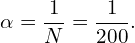
$\forall a,\quad\pi_a \leftarrow \pi_a + \alpha \frac{r_k}{v}\begin{cases}1 - \pi_a & \text{if } a = k, \-\pi_a & \text{otherwise.}\end{cases}$

$where (\alpha = 1/N)$

The swarm size is the learning rate. Bigger swarm, smaller step. The organism learns more slowly because there are more of them. That is not a bug. That is averaging. Pretty much the same physics as a learning rate.

You do not know the true mean rewards $(q)$ . So $(v)$ in the denominator is not an oracle. In any implementation that can actually run, $(v)$ is an online estimate. A moving average of rewards already seen. The normalization is “how good was this sample relative to what we have been getting.”

Skip the update when the estimate is sitting on zero. Do not divide by faith.

The continuous limit, and why the extra factor matters

Take the population large and the step small and you land on the Maynard-Smith replicator dynamic:

$\dot{\pi}_a = \frac{\pi_a}{v^{\pi}}\bigl(q_a^{\pi} - v^{\pi}\bigr),\qquad q_a^{\pi} = \mathbb{E}[r_a].$

Classic Cross Learning, pushed to the same limit, gives you the Taylor replicator:

$\dot{\pi}_a = \pi_a \bigl(q_a^{\pi} - v^{\pi}\bigr).$

The only new object is $(1/v^{\pi})$ . Absolute rewards wander. Noise wanders with them. Dividing by the current average value keeps the step from blowing up when every site is paying well and from stalling when every site is paying poorly. It is a baseline. Bees did not call it a baseline. The algebra does.

The paper’s conditions for reliable convergence include a neighborhood that is not tiny. Something like $(M \ge 5)$ before the quorum story gets trustworthy. Local does not mean “talk to one neighbor and call it wisdom.” Local means “small relative to $(N)$ , large enough to estimate a vote.” Hold that sentence. The plots below will test your patience.

One agent, N environments

Read the micro-rule from the macro side and the RL picture snaps into focus.

Each bee samples an action from $(\pi)$ . That is her current preference.
She receives a noisy reward from her own site visit. That is one environment.
Imitation averages those samples into the next $(\pi)$ .

That is a single online bandit agent aggregating action-value samples from $(N)$ parallel environments. The individuals are not learners in the gradient sense. They are samplers with a copy rule. The learner is the distribution.

i want to be careful about the evolutionary sentence, because it is the one people will over-claim( omg lets anthropormoisize yet another algorithm). The equivalence supplies a plausible selective pressure for the imitation rule: a group that copies this way is doing group-level reinforcement learning whether or not any bee could tell you that. The paper does not prove that kin selection “favors group-level RL” as a primary result. It shows you a mechanism that would be worth keeping if selection ever got its hands on it. Mechanism first. Story second.

Why i care, and why you might

Most “swarm intelligence” (papers, decks, napkins) still hand you a metaphor and a video of drones in a pretty formation. This hands you a pseudo-compiler. If you know which bandit update you want at the macro scale, you can ask what local imitation rule realizes it. If you already have a local rule, you can ask which RL agent you accidentally built.

That is a design tool. Drone search. Sensor tasking and orchestration. Any flock of cheap agents that should not each be running a policy network. You do not put a sophisticated learner in every airframe. You put a sampler and a dance in every airframe, and you let the population be the learner.

Same mathematics, opposite direction of work. Derive the local rule from the update you want. Or read the update off the rule you already shipped.

The notebook:

# Maynard-Cross Learning: one abstract agent, and the bees it claims to be.
# Soma, Bouteiller, Hamann, Beltrame — arXiv:2410.17517
#
# Macro: streaming MCL. One sample per step. Learning rate alpha = 1/N.
#        v is NOT the true mean reward. It is an exponential moving average
#        of rewards actually observed. That is the version you can ship.
#
# Hive:  N agents. Each holds a discrete site preference.
#        Each step, every agent hears M neighbors and copies with
#        probability proportional to the rewards those neighbors just drew.
#        Nobody stores pi. The histogram of preferences is pi.

import numpy as np
import matplotlib.pyplot as plt

# --- bandit and swarm ---
K = 5            # sites / arms
N = 200          # bees; also sets alpha = 1/N on the macro side
T = 2500         # steps. clocks differ; see the post
delta = 0.15     # uniform noise half-width around each q_a
beta = 0.02      # EMA rate for the online baseline v
M = 8            # neighborhood size for the healthy hive
num_runs = 4     # macro seeds for the mean/std band
SEED = 42

q = np.linspace(0.25, 0.85, K)   # 0.25, 0.40, 0.55, 0.70, 0.85
optimal = int(np.argmax(q))      # arm 4


def run_mcl_macro(T=T, seed=0, q=q):
    """Serial MCL. One environment sample per tick."""
    local = np.random.default_rng(seed)
    alpha = 1.0 / N
    pi = np.ones(K) / K
    v_est = 0.0
    history = np.zeros((T, K))
    arms = np.arange(K)

    for t in range(T):
        history[t] = pi
        k = local.choice(K, p=pi)
        r = np.clip(local.uniform(q[k] - delta, q[k] + delta), 0.0, 1.0)

        # online baseline. first reward seeds it; after that, EMA.
        v_est = r if t == 0 else (1.0 - beta) * v_est + beta * r
        if v_est < 1e-8:
            continue

        # MCL: reinforce k by (1 - pi_k), decay every other arm by pi_a,
        # then scale by alpha * (r / v).
        update = alpha * (r / v_est) * np.where(arms == k, 1.0 - pi, -pi)
        pi = np.clip(pi + update, 0.0, None)
        total = pi.sum()
        pi = pi / total if total > 0.0 else np.ones(K) / K

    return history


def run_hive(T=T, seed=0, M=M, q=q):
    """Explicit bees. No policy vector. Histogram only."""
    local = np.random.default_rng(seed)
    prefs = local.integers(0, K, size=N)   # each bee's current site
    history = np.zeros((T, K))

    for t in range(T):
        counts = np.bincount(prefs, minlength=K).astype(float)
        history[t] = counts / N

        # every bee samples a noisy reward for the site she currently likes
        rewards = np.clip(
            local.uniform(q[prefs] - delta, q[prefs] + delta), 0.0, 1.0
        )

        # one neighborhood draw per bee, then a weighted copy
        new_prefs = prefs.copy()
        neigh = local.integers(0, N, size=(N, M))
        for i in range(N):
            js = neigh[i]
            votes = np.bincount(prefs[js], weights=rewards[js], minlength=K)
            total = votes.sum()
            if total > 0.0:
                new_prefs[i] = local.choice(K, p=votes / total)
        prefs = new_prefs

    return history


pi_macro = run_mcl_macro(seed=SEED)
pi_hive = run_hive(seed=SEED, M=8)
pi_hive_small = run_hive(seed=SEED, M=2)   # thin vote; easy bandit still locks

percent_opt = np.vstack([
    run_mcl_macro(seed=SEED + r)[:, optimal] * 100.0
    for r in range(num_runs)
])
mean_opt = percent_opt.mean(axis=0)
std_opt = percent_opt.std(axis=0)

# Figure 1 — full policy, both ontologies
fig, axes = plt.subplots(1, 2, figsize=(12, 5), sharey=True)
for a in range(K):
    axes[0].plot(pi_macro[:, a], label=f"arm {a}  q={q[a]:.2f}")
    axes[1].plot(pi_hive[:, a], label=f"arm {a}  q={q[a]:.2f}")
axes[0].set_title("Macro MCL (one abstract agent)")
axes[1].set_title(f"Hive (N={N} bees, neighborhood M={M})")
for ax in axes:
    ax.set_xlabel("step")
    ax.set_ylabel(r"policy mass ")
    ax.set_ylim(0, 1.02)
    ax.grid(True, alpha=0.3)
    ax.legend(fontsize=8, loc="center right")
fig.tight_layout()
fig.savefig("mcl_policy_evolution.png", dpi=140)

# Figure 2 — mass on the best arm, plus a too-easy small neighborhood
fig, ax = plt.subplots(figsize=(12, 5.5))
ax.plot(pi_macro[:, optimal] * 100.0, color="C0", lw=2.0, label="Macro MCL (this seed)")
ax.plot(pi_hive[:, optimal] * 100.0, color="C1", lw=2.0, label="Hive, M=8")
ax.plot(pi_hive_small[:, optimal] * 100.0, color="C3", lw=1.6, label="Hive, M=2 (too local)")
ax.plot(mean_opt, color="black", lw=1.4, ls="--", label=f"Macro mean over {num_runs} seeds")
ax.fill_between(
    np.arange(T), mean_opt - std_opt, mean_opt + std_opt,
    color="0.2", alpha=0.15, label="macro +/- 1 std",
)
ax.set_xlabel("step")
ax.set_ylabel("percent of mass on the best arm")
ax.set_title("Same bandit, three stories: abstract update, healthy hive, thin vote")
ax.set_ylim(0, 105)
ax.grid(True, alpha=0.3)
ax.legend(loc="center right", fontsize=9)
fig.tight_layout()
fig.savefig("mcl_optimal_convergence.png", dpi=140)
plt.show()

print(f"final macro   {pi_macro[-1, optimal]:.3f}")
print(f"final hive M8 {pi_hive[-1, optimal]:.3f}")
print(f"final hive M2 {pi_hive_small[-1, optimal]:.3f}")

Ok what is all of this doing?

On this seed the final mass on the best arm is 0.952 for the abstract MCL agent, 1.000 for the hive with (M=8), and 1.000 for the hive with (M=2).

That is exactly what the plots show. The abstract agent converges steadily. The hive converges “violently”. (Ya know you have to have some human adjective for code or a storm).

If your hive runs slower, change the problem before you change the theory. Shrink the reward gap. Increase the noise. Make the vote harder. That is the next experiment. If the macro agent converges toward the best arm and the hive does not under the same reward structure, then look at the voting implementation first. The equivalence is not rescued or refuted by a bad bincount.

A batch macro update would give you the fairer clock: draw $(B=N)$ actions from $(\pi)$ , collect $(N)$ rewards, average the MCL increments, and apply the aggregate update once. At that point the blue macro curve should stop looking quite so lazy.

Note your probably wondering why not use DEAP? It is the wrong first tool. Nothing here is evolving a genome or code base. This is a probability distribution concentrating under reinforcement. If, later, you want to evolve the dance itself so that a local swarm rule realizes some other desired macro-level bandit update, then put run_hive inside a fitness function and evolve the microscopic rule. Different experiment. Different blog. Maybe sometime in the future.

This one is the equivalence, watched with the lights on cause i’d rather see bees than hear them.

What the run actually did

Five arms. Mean rewards:

$q = (0.25,\ 0.40,\ 0.55,\ 0.70,\ 0.85).$

Uniform reward noise has half-width

$\delta = 0.15,$

with samples clipped to ([0,1]).

Arm 4 is optimal with expected reward (q_4=0.85).

The swarm contains

$N=200$

bees, which also sets the serial macro learning rate to

$\alpha = \frac{1}{N}=\frac{1}{200}.$

The online value baseline uses an exponential moving average with

$\beta = 0.02.$

The run lasts (T=2500) steps. The healthy hive uses a neighborhood size (M=8). A second hive uses (M=2). We repeat the macro comparison across four seeds.

Same bandit. Same reward noise. Same initial ignorance. Very different clocks.

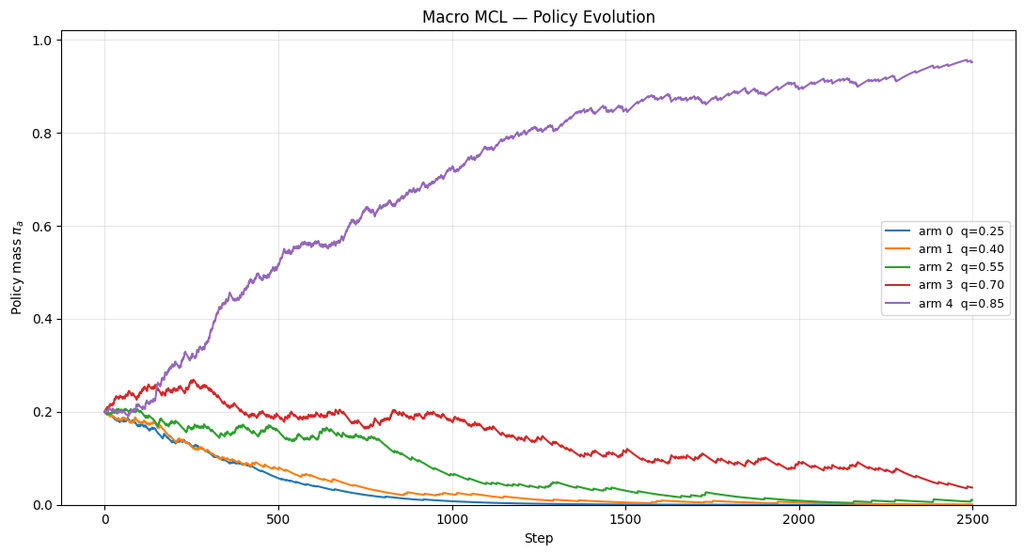
Figure 1 — Macro MCL policy evolution

The abstract MCL agent begins uniformly:

$\pi_a = 0.2$

for all five arms.

From there, arm 4 starts accumulating mass while the weaker alternatives are progressively starved.

The movement is not monotonic because the agent is sampling noisy rewards one observation at a time. Arm 3, with (q=0.70), survives longest because it is the nearest competitor. The lower-reward arms disappear much earlier.

For the seed shown:

around step 100, arm 4 holds (0.213) of the policy;
around step 500, it holds (0.518);
around step 1000, it holds (0.725);
at step 2499, it holds (0.952).

Across the four macro seeds, the final mass on arm 4 ranges from approximately (91.5%) to (97.9%), with a final mean of (95.2%) and a standard deviation of about (2.37) percentage points.

The walk is noisy. The destination is not (which is usually always the case in life).

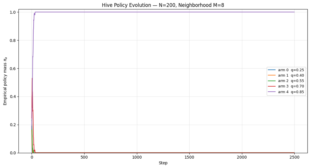
Figure 2 — Hive policy evolution, (M=8)

The hive is doing something operationally very different. This is a test of the public bee broadcasting system this is only a test.

There is no global $(\pi)$ stored anywhere. Will we converge? The suspense is killing me i hope it lasts!

Each bee carries only a discrete site preference. Each bee samples a noisy reward from that site. Each bee then looks at (M=8) randomly selected neighbors and copies a site according to the neighbors’ reward-weighted votes. The policy exists only as the histogram of those preferences. And that histogram locks fast.

With (N=200) and (M=8), the optimal arm exceeds (95%) of the population by about step 22, exceeds (99%) by about step 24, and reaches complete fixation by about step 33.

The other four traces collapse onto the floor. That does not mean the hive discovered a better learning rule. It means the hive is consuming much more information per tick (i’m not sure if that is the correct wording; you can’t consume information?). The serial macro loop samples one action and one reward per step.

The hive samples roughly (N=200) rewards and performs roughly (N=200) local imitation decisions per step. Same family of mathematics. Very different amount of work per tick.

That distinction matters.

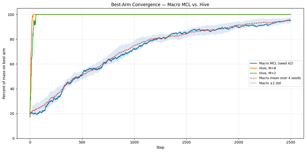
Figure 3 — Best-arm convergence

The convergence plot makes the clock mismatch explicit.

Blue is the serial Macro MCL run for seed 42.
Orange is the hive with (M=8).
Green is the hive with (M=2).
The dashed red line is the mean of the four macro runs.
The shaded band is $(\pm 1)$ standard deviation across those macro runs.

Both hive variants race to the ceiling while the macro agent climbs gradually toward the same winner.

The (M=8) hive reaches complete fixation at roughly step 33.

The (M=2) hive takes longer, but only slightly: it exceeds (95%) around step 37 and reaches complete fixation around step 58.

So on this particular bandit, (M=2) does not fail.

That is important.

The reward means are spaced by (0.15), and the noise half-width is also (0.15). Arm 4 is sufficiently better than the alternatives that even a very thin neighborhood vote usually discovers the correct direction.

The paper’s warning about very small neighborhoods concerns reliability when the alternatives are harder to distinguish: smaller reward gaps, heavier noise, or situations where a lucky local sample can pull a tiny neighborhood into premature consensus. That is the experiment to run next. Let’s Shrink the gap.

Now let us increase $(\delta)$ .

Then see whether (M=2) starts believing the first charismatic (tiny) dancer it meets. Hold me close. Get the lyric?

Figure 4 — Early-time convergence

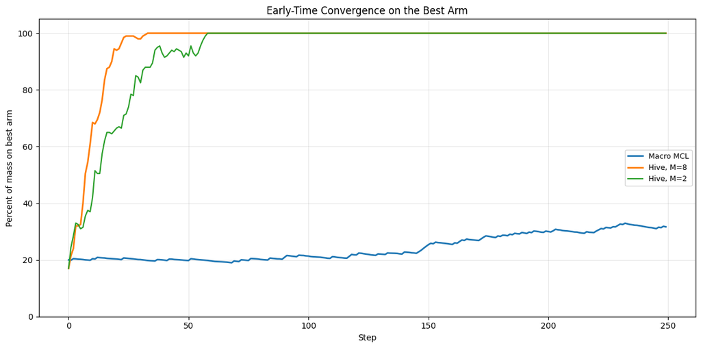
The early-time zoom is probably the clearest picture in the set because it removes the long flat tail after the hive has already converged. Within the first 250 steps, the distinction is obvious.

The (M=8) hive climbs from roughly (20%) initial representation to complete fixation in only a few dozen collective updates.

The (M=2) hive is somewhat noisier and slower, but still reaches fixation before step 60.

Over the same interval, the serial macro agent is still wandering between roughly (20%) and (30%) policy mass on the optimal arm.

Again: do not read that as intelligence. Read the clock. One side is processing one reward sample per tick. The other side is processing a population-sized batch. The comparison is deliberately unfair in wall-clock information because that unfairness exposes the architecture.

If you want schedule equivalence, batch the macro learner with (B=N), or slow the hive down to one imitation event per tick. What the plots show cleanly is something narrower and more interesting: the abstract update and the swarm of local copiers select the same arm. They agree on the destination. They do not agree on the schedule. The destination is the mathematical equivalence. The schedule is an implementation choice.

Confusing those two is like looking at the orange line, looking at the blue line, and deciding the theorem must be wrong because one of them has a faster clock.

The early-convergence zoom is particularly useful because it makes the clock mismatch visually obvious: the hive gets essentially to 100% within tens of collective updates while serial MCL is still around 20–30%. That directly illustrates the explanation that the “macro loop” consumes one reward per tick while the hive is consuming roughly $(N)$ fresh observations per collective tick

Broader Implications For Maynard Learning

A swarm of cheap physical agents does not need a genius in every airframe. The paper’s equivalence says the opposite: if each body only samples and imitates locally, the population itself is already one online learner, aggregating noisy rewards across many parallel environments. In defense tech and physical AI that is a design rule, not a metaphor. A flock of scouts, buoys, or small unmanned vehicles can search, sense, and commit to a site, a route, or a task by a weighted-voter dance whose macro-update is Maynard-Cross Learning, with learning rate set by how many bodies you field and with no central policy server in the loop. Individuals stay simple, sometimes even “irrational” if you grade them one at a time. The group still converges. You get scale, you lose the single radio that everyone is waiting on, and you design the local copy rule so the hive you actually built is the bandit agent you meant to field.

It challenges traditional views of “intelligence” (the stochastic parrots will tell you they are) as individual-centric, showing how distributed systems can rival advanced RL agents through emergence.

Until Then,

#iwishyouwater <- the swarm does not have a leader. West Palm Beach Doing THE THANG.

#EverForward, stay local and still converge.

𝕋𝕖𝕕 ℂ. 𝕋𝕒𝕟𝕟𝕖𝕣 𝕁𝕣. (@tctjr) / X

MUZAK TO BLOG BY: Madman Across The Water, Tiny Dancer. Of course, Bernie Taupin was a lyrical genius, and well, you go play and sing like the madman – hold me closer, Tiny Dancer. Then i thought maybe Choo Choo Cha Choo? I am he, As you are he, As you are me, And we are all together, convergence if you will. The Oingo Boingo version is fire. Then again there is no one like the original.

Footnotes

[1] John Maynard Smith founded the ESS idea. The continuous replicator equation came later (Taylor & Jonker; Schuster & Sigmund). ESS is what the dynamics often sit down on. Do not hand him the differential equation. He already has enough credit. John Maynard Smith is also recognized as the founder of evolutionary game theory, providing the essential framework and the ESS concept that underpins the field, which later researchers, including those who formulated replicator dynamics, built upon. While Maynard Smith’s initial work focused on the static equilibrium concept of ESS, the replicator dynamics is a related concept developed later by other researchers (notably Taylor and Jonker, and Schuster and Sigmund) to describe the process of how strategies change in a population over time. The replicator equation is a set of differential equations that models how the frequency of a given strategy increases if its payoff (fitness) is higher than the average payoff of the population. The ESS is the stable, stationary point that the replicator dynamics often converge to.

[2] Cross Learning is the “imitation of success” aggregate. MCL is the weighted-voter aggregate. Same family, different micro-rule, different $(1/v)$ in the limit. If you implement CL by deleting the division, you can watch the robustness claim instead of taking my word for it.

[3] IS IT still ok to use jupyter notebooks? Is it like bell bottoms that might come back into vogue one day?

[4] Is it straight edge or punk to write your own LATEX?

[5] Hat tip to Fiona Cashin, keep those bees healthy. Great talking to you.

August 3, 2025August 3, 2025 TCTJr Artificial_Intelligence|Complexity_Theory|Distributed_Computing|Mathematics|Random_Thoughts

A Survey Of Architectures And Methodologies For Distributed LLM Dissaggregation

Grok 4’s Idea of a Distributed LLM

I was kicking back in my Charleston study this morning, drinking my usual unsweetened tea in a mason jar, the salty breeze slipping through the open window like a whisper from the Charleston Harbor, carrying that familiar tang of low tide “pluff mud” and distant rain. The sun was filtering through the shutters, casting long shadows across my desk littered with old notes on distributed systems engineering, when I dove into this survey on architectures for distributed LLM disaggregation. It’s a dive into the tech that’s pushing LLMs beyond their limits. As i read the numerous papers and assembled commonalities, it hit me how these innovations echo the battles many have fought scaling AI/ML in production, raw, efficient, and unapologetically forward. Here’s the breakdown, with the key papers linked for those ready to dig deeper.

This is essentially the last article in a trilogy. The sister survey is a blog A Survey of Technical Approaches For Distributed AI In Sensor Networks. Then, for a top-level view, i wrote SnakeByte[21]: The Token Arms Race: Architectures Behind Long-Context Foundation Models, so you’ll have all views of a complete system, sensors->distributed compute methods->context engineering.

NOTE: By the time this is published, a whole new set of papers will come out, and i wrote (and read the papers) in a week.

Overview

Distributed serving of LLMs presents significant technical challenges driven by the immense scale of contemporary models, the computational intensity of inference, the autoregressive nature of token generation, and the diverse characteristics of inference requests. Efficiently deploying LLMs across clusters of hardware accelerators (predominantly GPUs and NPUs) necessitates sophisticated system architectures, scheduling algorithms, and resource management techniques to achieve low latency, high throughput, and cost-effectiveness while adhering to Service Level Objectives (SLOs). As you read the LLM survey, think in terms of deployment architectures:

Layered AI System Architecture:

Sensor Layer: IoT, Cameras, Radar, LIDAR, electro-mag, FLIR etc
Edge/Fog Layer: Edge Gateways, Inference Accelerators, Fog Nodes
Cloud Layer: Central AI Model Training, Orchestration Logic, Data Lake

Each layer plays a role in collecting, processing, and managing AI workloads in a distributed system.

Distributed System Architectures and Disaggregation

Modern distributed Large Language Models serving platforms are moving beyond monolithic deployments to adopt disaggregated architectures. A common approach involves separating the computationally intensive prompt processing (prefill phase) from the memory-bound token generation (decode phase). This disaggregation addresses the bimodal latency characteristics of these phases, mitigating pipeline bubbles that arise in pipeline-parallel deployments KV-cache Streaming for Fast, Fault-tolerant Generative LLM Serving. As a reminder in LLMs, KV cache stores key and value tensors from previous tokens during inference. In transformer-based models, the attention mechanism computes key (K) and value (V) vectors for each token in the input sequence. Without caching, these would be recalculated for every new token generated, leading to redundant computations and inefficiency.

Systems like Mooncake: A KVCache-centric Disaggregated Architecture for LLM Serving propose a KVCache-centric disaggregated architecture with dedicated clusters for prefill and decoding. This separation allows for specialized resource allocation and scheduling policies tailored to each phase’s demands. Similarly, P/D-Serve: Serving Disaggregated Large Language Model at Scale focuses on serving disaggregated LLMs at scale across tens of thousands of devices, emphasizing fine-grained P/D organization and dynamic ratio adjustments to minimize inner mismatch and improve throughput and Time-to-First-Token (TTFT) SLOs. KVDirect: Distributed Disaggregated LLM Inference explores distributed disaggregated inference by optimizing inter-node KV cache transfer using tensor-centric communication and a pull-based strategy.

Further granularity in disaggregation can involve partitioning the model itself across different devices or even separating attention layers, as explored by Infinite-LLM: Efficient LLM Service for Long Context with DistAttention and Distributed KVCache, which disaggregates attention layers to enable flexible resource scheduling and enhance memory utilization for long contexts. DynaServe: Unified and Elastic Execution for Dynamic Disaggregated LLM Serving unifies and extends both colocated and disaggregated paradigms using a micro-request abstraction, splitting requests into segments for balanced load across unified GPU instances.

The distributed nature also necessitates mechanisms for efficient checkpoint loading and live migration. ServerlessLLM: Low-Latency Serverless Inference for Large Language Models proposes a system for low-latency serverless inference that leverages near-GPU storage for fast multi-tier checkpoint loading and supports efficient live migration of LLM inference states.

Scheduling and Resource Orchestration

Effective scheduling is paramount in distributed LLM serving due to heterogeneous request patterns, varying SLOs, and the autoregressive dependency. Existing systems often suffer from head-of-line blocking and inefficient resource utilization under diverse workloads.

Preemptive scheduling, as implemented in Fast Distributed Inference Serving for Large Language Models, allows for preemption at the granularity of individual output tokens to minimize latency. FastServe employs a novel skip-join Multi-Level Feedback Queue scheduler leveraging input length information. Llumnix: Dynamic Scheduling for Large Language Model Serving introduces dynamic rescheduling across multiple model instances, akin to OS context switching, to improve load balancing, isolation, and prioritize requests with different SLOs via an efficient live migration mechanism.

Prompt scheduling with KV state sharing is a key optimization for workloads with repetitive prefixes. Preble: Efficient Distributed Prompt Scheduling for LLM Serving is a distributed platform explicitly designed for optimizing prompt sharing through a distributed scheduling system that co-optimizes KV state reuse and computation load-balancing using a hierarchical mechanism. MemServe: Context Caching for Disaggregated LLM Serving with Elastic Memory Pool integrates context caching with disaggregated inference, supported by a global scheduler that enhances cache reuse through a global prompt tree-based locality-aware policy. Locality-aware fair scheduling is further explored in Locality-aware Fair Scheduling in LLM Serving, which proposes Deficit Longest Prefix Match (DLPM) and Double Deficit LPM (D2LPM) algorithms for distributed setups to balance fairness, locality, and load-balancing.

Serving multi-SLO requests efficiently requires sophisticated queue management and scheduling. Queue management for slo-oriented large language model serving is a queue management system that handles batch and interactive requests across different models and SLOs using a Request Waiting Time (RWT) Estimator and a global scheduler for orchestration. SLOs-Serve: Optimized Serving of Multi-SLO LLMs optimizes the serving of multi-stage LLM requests with application- and stage-specific SLOs by customizing token allocations using a multi-SLO dynamic programming algorithm. SeaLLM: Service-Aware and Latency-Optimized Resource Sharing for Large Language Model Inference proposes a service-aware and latency-optimized resource sharing framework for large language model inference.

For complex workloads like agentic programs involving multiple LLM calls with dependencies, traditional request-level scheduling is suboptimal. Autellix: An Efficient Serving Engine for LLM Agents as General Programs treats programs as first-class citizens, using program-level context to inform scheduling algorithms that preempt and prioritize LLM calls based on program progress, demonstrating significant throughput improvements for agentic workloads. Parrot: Efficient Serving of LLM-based Applications with Semantic Variable focuses on end-to-end performance for LLM-based applications by introducing the Semantic Variable abstraction to expose application-level knowledge and enable data flow analysis across requests. Conveyor: Efficient Tool-aware LLM Serving with Tool Partial Execution optimizes for tool-aware LLM serving by enabling tool partial execution alongside LLM decoding.

Memory Management and KV Cache Optimizations

The KV cache’s size grows linearly with sequence length and batch size, becoming a major bottleneck for GPU memory and throughput. Distributed serving exacerbates this by requiring efficient management across multiple nodes.

Effective KV cache management involves techniques like dynamic memory allocation, swapping, compression, and sharing. KV-cache Streaming for Fast, Fault-tolerant Generative LLM Serving proposes KV-cache streaming for fast, fault-tolerant serving, addressing GPU memory overprovisioning and recovery times. It utilizes microbatch swapping for efficient GPU memory management. On-Device Language Models: A Comprehensive Review presents techniques for managing persistent KV cache states including tolerance-aware compression, IO-recompute pipelined loading, and optimized chunk lifecycle management.

In distributed environments, sharing and transferring KV cache states efficiently are critical. MemServe introduces MemPool, an elastic memory pool managing distributed memory and KV caches. Infinite-LLM: Efficient LLM Service for Long Context with DistAttention and Distributed KVCache leverages a pooled GPU memory strategy across a cluster. Prefetching KV-cache for LLM Inference with Dynamic Profiling proposes prefetching model weights and KV-cache from off-chip memory to on-chip cache during communication to mitigate memory bottlenecks and communication overhead in distributed settings. KVDirect: Distributed Disaggregated LLM Inference specifically optimizes KV cache transfer using a tensor-centric communication mechanism.

Handling Heterogeneity and Edge/Geo-Distributed Deployment

Serving LLMs cost-effectively often requires utilizing heterogeneous hardware clusters and deploying models closer to users on edge devices or across geo-distributed infrastructure.

Helix: Serving Large Language Models over Heterogeneous GPUs and Networks via Max-Flow addresses serving LLMs over heterogeneous GPUs and networks by formulating inference as a max-flow problem and using MILP for joint model placement and request scheduling optimization. LLM-PQ: Serving LLM on Heterogeneous Clusters with Phase-Aware Partition and Adaptive Quantization supports efficient serving on heterogeneous GPU clusters through adaptive model quantization and phase-aware partition. Efficient LLM Inference via Collaborative Edge Computing leverages collaborative edge computing to partition LLM models and deploy them on distributed devices, formulating device selection and partition as an optimization problem.

Deploying LLMs on edge or geo-distributed devices introduces challenges related to limited resources, unstable networks, and privacy. PerLLM: Personalized Inference Scheduling with Edge-Cloud Collaboration for Diverse LLM Services provides a personalized inference scheduling framework with edge-cloud collaboration for diverse LLM services, optimizing scheduling and resource allocation using a UCB algorithm with constraint satisfaction. Distributed Inference and Fine-tuning of Large Language Models Over The Internet investigates inference and fine-tuning over the internet using geodistributed devices, developing fault-tolerant inference algorithms and load-balancing protocols. MoLink: Distributed and Efficient Serving Framework for Large Models is a distributed serving system designed for heterogeneous and weakly connected consumer-grade GPUs, incorporating techniques for efficient serving under limited network conditions. WiLLM: an Open Framework for LLM Services over Wireless Systems proposes deploying LLMs in core networks for wireless LLM services, introducing a “Tree-Branch-Fruit” network slicing architecture and enhanced slice orchestration.

On the of most recent papers that echo my sentiment from years ago where is i’ve said “Vertically Trained Horizontally Chained” (maybe i should trademark that …) is Small Language Models are the Future of Agentic AI where they lay out the position that specific task LLMs are sufficiently robust, inherently more suitable, and necessarily more economical for many invocations in agentic systems, and are therefore the future of agentic AI. The argumentation is grounded in the current level of capabilities exhibited by these specialized models, the common architectures of agentic systems, and the economy of LM deployment. They further argue that in situations where general-purpose conversational abilities are essential, heterogeneous agentic systems (i.e., agents invoking multiple different models chained horizontally) are the natural choice. They discuss the potential barriers for the adoption of vertically trained LLMs in agentic systems and outline a general LLM-to-specific chained model conversion algorithm.

Other Optimizations and Considerations

Quantization is a standard technique to reduce model size and computational requirements. Atom: Low-bit Quantization for Efficient and Accurate LLM Serving proposes a low-bit quantization method (4-bit weight-activation) to maximize serving throughput by leveraging low-bit operators and reducing memory consumption, achieving significant speedups over FP16 and INT8 with negligible accuracy loss.

Splitting or partitioning models can also facilitate deployment across distributed or heterogeneous resources. SplitLLM: Collaborative Inference of LLMs for Model Placement and Throughput Optimization designs a collaborative inference architecture between a server and clients to enable model placement and throughput optimization. A related concept is Split Learning for fine-tuning, where models are split across cloud, edge, and user devices Hierarchical Split Learning for Large Language Model over Wireless Network. BlockLLM: Multi-tenant Finer-grained Serving for Large Language Models enables multi-tenant finer-grained serving by partitioning models into blocks, allowing component sharing, adaptive assembly, and per-block resource configuration.

Performance and Evaluation Metrics

Evaluating and comparing distributed LLM serving platforms requires appropriate metrics and benchmarks. The CAP Principle for LLM Serving: A Survey of Long-Context Large Language Model Serving suggests a trade-off between serving context length (C), serving accuracy (A), and serving performance (P). Developing realistic workloads and simulation tools is crucial. BurstGPT: A Real-world Workload Dataset to Optimize LLM Serving Systems provides a real-world workload dataset for optimizing LLM serving systems, revealing limitations of current optimizations under realistic conditions. LLMServingSim: A HW/SW Co-Simulation Infrastructure for LLM Inference Serving at Scale is a HW/SW co-simulation infrastructure designed to model dynamic workload variations and heterogeneous processor behaviors efficiently. ScaleLLM: A Resource-Frugal LLM Serving Framework by Optimizing End-to-End Efficiency focuses on a holistic system view to optimize LLM serving in an end-to-end manner, identifying and addressing bottlenecks beyond just LLM inference.

Conclusion

The landscape of distributed LLM serving platforms is rapidly evolving, driven by the need to efficiently and cost-effectively deploy increasingly large and complex models. Key areas of innovation include the adoption of disaggregated architectures, sophisticated scheduling algorithms that account for workload heterogeneity and SLOs, advanced KV cache management techniques, and strategies for leveraging diverse hardware and deployment environments. While significant progress has been made, challenges remain in achieving optimal trade-offs between performance, cost, and quality of service (QOS) across highly dynamic and heterogeneous real-world scenarios.

As the sun set and the neon glow of my screen dimmed, i wrapped this survey up, leaving me pondering the endless horizons of AI/ML scaling like waves crashing on the shore, relentless and full of promise and thinking how incredible it is to be working in these areas where what we have dreamed for decades has come to fruition?

Until Then,

#iwishyouwater

Ted ℂ. Tanner Jr. (@tctjr) / X

MUZAK TO BLOG BY: Vangelis, “L’apocalypse de animax (remastered). Vangelis is famous for “Chariots Of Fire” and “Blade Runner” Soundtracks.

A Survey of Technical Approaches For Distributed AI In Sensor Networks

Grok4’s Idea of AI and Sensor Orchestraton with DAI

Distributed Artificial Intelligence (DAI) within sensor networks (SN) involves deploying AI algorithms and models across a network of spatially distributed sensor nodes rather than relying solely on centralized cloud processing. This paradigm shifts computation closer to the data source, bringing the data to the compute, offering potential benefits in terms of reduced communication latency, lower bandwidth usage, enhanced privacy, increased system resilience, and improved scalability for large-scale IoT and pervasive computing deployments. The operational complexity of such systems necessitates sophisticated orchestration mechanisms to manage the distributed AI workloads, sensor resources, and heterogeneous compute infrastructure spanning from edge devices to cloud data centers. This article will survey methods for distributed smart sensor technologies, along with considerations for implementing AI algorithms at these junctions.

Implementing AI functions in a distributed sensor network setting often involves adapting centralized algorithms or devising novel distributed methods. Key technical areas include distributed estimation, detection, and learning.

Distributed Sensor Anomaly Detection

Distributed estimation problems, such as static parameter estimation or Kalman filtering, can be addressed using consensus-based approaches. Algorithms of the “consensus + innovations” type, where one can have an estimation of the type and behavior of the sensor. The paper “Distributed Parameter Estimation in Sensor Networks: Nonlinear Observation Models and Imperfect Communication” discusses these algorithms, which enable sensor nodes to iteratively update estimates by combining local observations (innovations) with information exchanged with neighbors (consensus). These methods enable asymptotically unbiased and efficient estimation, even in the presence of nonlinear observation models and imperfect communication. Extensions include randomized consensus for Kalman filtering, which offers robustness to network topology changes and distributes the computational load stochastically which are covered in the paper “Randomized Consensus based Distributed Kalman Filtering over Wireless Sensor Networks”. For multi-target tracking or target under consideration, distributed approaches integrate sensor registration with tracking filters, such as deploying a consensus cardinality probability hypothesis density (CPHD) filter across the network and minimizing a cost function based on local posteriors to estimate relative sensor poses in the paper “Distributed Joint Sensor Registration and Multitarget Tracking Via Sensor Network”.

Distributed detection focuses on identifying events or anomalies based on collective sensor readings. Techniques leveraging sparse signal recovery have been applied to detect defective sensors in networks with a small number of faulty nodes, using distributed iterative hard thresholding (IHT) and low-complexity decoding robust to noisy messages in these two papers “Distributed Sparse Signal Recovery For Sensor Networks” and “Distributed Sensor Failure Detection In Sensor Networks” cover methods for failure recovery and self healing.

In another closely related application for anomaly detection of sensors learning-based distributed procedures, like the mixed detection-estimation (MDE) algorithm, address scenarios with unknown sensor defects by iteratively learning the validity of local observations while refining parameter estimates, achieving performance close to ideal centralized estimators in high SNR regimes can be found in this paper “Learning-Based Distributed Detection-Estimation in Sensor Networks with Unknown Sensor Defects”.

Distributed learning enables sensor nodes or edge devices to collaboratively train models without requiring the sharing of raw data. This is crucial for maintaining privacy and conserving bandwidth, or where privacy-preserving machine learning (PPML) is necessary. Approaches include distributed dictionary learning using diffusion cooperation schemes, where nodes exchange local dictionaries with neighbors, are applied in this paper “Distributed Dictionary Learning Over A Sensor Network”

In many cases, one has no a priori information for the type of sensor under consideration. For online sensor selection with unknown utility functions, distributed online greedy (DOG) algorithms provide no-regret guarantees for submodular utility functions with minimal communication overhead. Federated Learning (FL) and other distributed Machine Learning (ML) paradigms are increasingly applied for tasks like anomaly detection. In the paper “ Online Distributed Sensor Selection,” we find that a key problem in sensor networks is to decide which sensors to query when, in order to obtain the most useful information (e.g., for performing accurate prediction), subject to constraints (e.g., on power and bandwidth). In many applications, the utility function is not known a priori, must be learned from data, and can even change over time. Furthermore, for large sensor networks, solving a centralized optimization problem to select sensors is not feasible, and thus we seek a fully distributed solution. In most cases, training on raw data occurs locally, and model updates or parameters are aggregated globally, often at an edge server or fusion center.

Sensor activation and selection are also critical aspects. Forward-thinking algorithms in energy-efficient distributed sensor activation based on predicted target locations using computational intelligence can significantly reduce energy consumption and the number of active nodes required for target tracking such as the paper IDSA: Intelligent Distributed Sensor Activation Algorithm For Target Tracking With Wireless Sensor Network.

Context-aware like those that are emerging with Large Language Models, can collaborate with intelligence and in-sensor analytics (ISA) on resource-constrained nodes, dramatically reducing communication energy compared to transmitting raw data, extending network lifetime while preserving essential information

Context-Aware Collaborative-Intelligence with Spatio-Temporal In-Sensor-Analytics in a Large-Area IoT Testbed introduces a context-aware collaborative-intelligence approach that incorporates spatio-temporal in-sensor analytics (ISA) to reduce communication energy in resource-constrained IoT nodes. This approach is particularly relevant given that energy-efficient communication remains a primary bottleneck in achieving fully energy-autonomous IoT nodes, despite advancements in reducing the energy cost of computation. The research explores the trade-offs between communication and computation energies in a mesh network deployed across a large-scale university campus, targeting multi-sensor measurements for smart agriculture (temperature, humidity, and water nitrate concentration).

The paper considers several scenarios involving ISA, Collaborative Intelligence (CI), and Context-Aware-Switching (CAS) of the cluster-head during CI. A real-time co-optimization algorithm is developed to minimize energy consumption and maximize the battery lifetime of individual nodes. The results show that ISA consumes significantly less energy compared to traditional communication methods: approximately 467 times lower than Bluetooth Low Energy (BLE) and 69,500 times lower than Long Range (LoRa) communication. When ISA is used in conjunction with LoRa, the node lifetime increases dramatically from 4.3 hours to 66.6 days using a 230 mAh coin cell battery, while preserving over 98% of the total information. Furthermore, CI and CAS algorithms extend the worst-case node lifetime by an additional 50%, achieving an overall network lifetime of approximately 104 days, which is over 90% of the theoretical limits imposed by leakage currents.

Orchestration of Distributed AI and Sensor Resources

Orchestration in the context of distributed AI and sensor networks involves the automated deployment, configuration, management, and coordination of applications, dataflows, and computational resources across a heterogeneous computing continuum, typically spanning sensors, edge devices, fog nodes, and the cloud. The paper Orchestration in the Cloud-to-Things Compute Continuum: Taxonomy, Survey and Future Directions. This is essential for supporting complex, dynamic, and resource-intensive AI workloads in pervasive environments.

Traditional orchestration systems designed for centralized cloud environments are often ill-suited for the dynamic and resource-constrained nature of edge/fog computing and sensor networks. Requirements for continuum orchestration include support for diverse data models (streams, micro-batches), interfacing with various runtime engines (e.g., TensorFlow), managing application lifecycles (including container-based deployment), resource scheduling, and dynamic task migration.

Container orchestration tools, widely used in cloud environments, are being adapted for edge and fog computing to manage distributed containerized applications. However, deploying heavy-weight orchestrators on resource-limited edge/fog nodes presents challenges. Lightweight container orchestration solutions, such as clusters based on K3s, are proposed to support hybrid environments comprising heterogeneous edge, fog, and cloud nodes, offering improved response times for real-time IoT applications. The paper Container Orchestration in Edge and Fog Computing Environments for Real-Time IoT Applications proposes a feasible approach to build a hybrid and lightweight cluster based on K3s, a certified Kubernetes distribution for constrained environments that offers containerized resource management framework. This work addresses the challenge of creating lightweight computing clusters in hybrid computing environments. It also proposes three design patterns for the deployment of the “FogBus2” framework in hybrid environments, including 1) Host Network, 2) Proxy Server, and 3) Environment Variable.

Machine learning algorithms are increasingly integrated into container orchestration systems to improve resource provisioning decisions based on predicted workload behavior and environmental conditions where it is mentioned in the paper ECHO: An Adaptive Orchestration Platform for Hybrid Dataflows across Cloud and Edge with an open source model.

Platforms like ECHO are designed to orchestrate hybrid dataflows across distributed cloud and edge resources, enabling applications such as video analytics and sensor stream processing on diverse hardware platforms. Other frameworks such as the paper DAG-based Task Orchestration for Edge Computing, focus on orchestrating application tasks with dependencies (represented as Directed Acyclic Graphs, or DAGs) on heterogeneous edge devices, including personally owned, unmanaged devices, to minimize end-to-end latency and reduce failure probability. Of note, this is also closely aligned with implementations of MFLow and Airflow, which implement a DAG.

Autonomic orchestration aims to create self-managing distributed systems. This involves using AI, particularly edge AI, to enable local autonomy and intelligence in resource orchestration across the device-edge-cloud continuum as discussed in Autonomy and Intelligence in the Computing Continuum: Challenges, Enablers, and Future Directions for Orchestration. For instance, in A Self-Managed Architecture for Sensor Networks Based on Real Time Data Analysis introduces a self-managed sensor network platforms that can use real-time data analysis to dynamically adjust network operations and optimize resource usage. AI-enabled traffic orchestration in future networks (e.g., 6G) utilizes technologies like digital twins to provide smart resource management and intelligent service provisioning for complex services like ultra-reliable low-latency communication (URLLC) and distributed AI workflows. There is an underlying interplay between Distributed AI Workflow and URLLC, which has manifold design considerations throughout any network topology.

Novel paradigms such as the paper How Can AI be Distributed in the Computing Continuum? Introducing the Neural Pub/Sub Paradigm are emerging to address the specific challenges of orchestrating large-scale distributed AI workflows. The neural publish/subscribe paradigm proposes a decentralized approach to managing AI training, fine-tuning, and inference workflows in the computing continuum, aiming to overcome limitations of traditional centralized brokers in handling the massive data surge from connected devices. This paradigm facilitates distributed computation, dynamic resource allocation, and system resilience. Similarly, concepts like Airborne Neural Networks envision distributing neural network computations across multiple airborne devices, coordinated by airborne controllers, for real-time learning and inference in aerospace applications found in the paper Airborne Neural Network. This paper proposes a novel concept: the Airborne Neural Network a distributed architecture where multiple airborne devices, each host a subset of neural network neurons. These devices compute collaboratively, guided by an airborne network controller and layer-specific controllers, enabling real-time learning and inference during flight. This approach has the potential to revolutionize Aerospace applications, including airborne air traffic control, real-time weather and geographical predictions, and dynamic geospatial data processing.

The intersection of distributed AI and sensor orchestration is also evident in specific applications like multi-robot systems for intelligence, surveillance, and reconnaissance (ISR), where decentralized coordination algorithms enable simultaneous exploration and exploitation in unknown environments using heterogeneous robot teams such as Decentralised Intelligence, Surveillance, and Reconnaissance in Unknown Environments with Heterogeneous Multi-Robot Systems, In the paper Coordination of Drones at Scale: Decentralized Energy-aware Swarm Intelligence for Spatio-temporal Sensing it is introduced a solution to tackle the complex task self-assignment problem, a decentralized and energy-aware coordination of drones at scale is introduced. Autonomous drones share information and allocate tasks cooperatively to meet complex sensing requirements while respecting battery constraints. Furthermore, the decentralized coordination method prevents single points of failure, it is more resilient, and preserves the autonomy of drones to choose how they navigate and sense. In the paper HiveMind: A Scalable and Serverless Coordination Control Platform for UAV Swarms, a centralized coordination control platform for IoT swarms is introduced that is both scalable and performant. HiveMind leverages a centralized cluster for all resource-intensive computation, deferring lightweight and time-critical operations, such as obstacle avoidance, to the edge devices to reduce network traffic. Resource orchestration for network slicing scenarios can employ distributed reinforcement learning (DRL) where multiple agents cooperate to dynamically allocate network resources based on slice requirements, demonstrating adaptability without extensive retraining found in the paper Using Distributed Reinforcement Learning for Resource Orchestration in a Network Slicing Scenario.

Challenges and Implementation Considerations

Implementing distributed AI and sensor orchestration presents numerous challenges:

Communication Constraints: The limited bandwidth, intermittent connectivity, and energy costs associated with wireless communication in sensor networks necessitate communication-efficient algorithms and data compression techniques. Distributed learning algorithms often focus on minimizing the number of communication rounds or the size of exchanged messages as discussed in Pervasive AI for IoT applications: A Survey on Resource-efficient Distributed Artificial Intelligence.

Computational Heterogeneity: Sensor nodes, edge devices, and cloud servers possess vastly different computational capabilities. Orchestration systems must effectively map AI tasks to appropriate resources, potentially offloading intensive computations to the edge or cloud while performing lightweight inference or pre-processing on resource-constrained nodes as found in Pervasive AI for IoT applications: A Survey on Resource-efficient Distributed Artificial Intelligence and further discussed a problems in Autonomy and Intelligence in the Computing Continuum: Challenges, Enablers, and Future Directions for Orchestration.

Resource Management: Dynamic allocation and optimization of compute, memory, storage, and network resources are critical for performance and efficiency, especially with fluctuating workloads and device availability in the paper Container Orchestration in Edge and Fog Computing Environments for Real-Time IoT Applications To orchestrate a multitude of containers, several orchestration tools are developed. But, many of these orchestration tools are heavy-weight and have a high overhead, especially for resource-limited Edge/Fog nodes

Fault Tolerance and Resilience: In A Distributed Architecture for Edge Service Orchestration with Guarantees it is discussed how istributed systems are prone to node failures, communication link disruptions, and dynamic changes in network topology affect global convergence. Algorithms and orchestration platforms must be designed to handle such uncertainties and ensure system availability and reliability.

Security and Privacy: Distributing data processing raises concerns about data privacy and model security. Federated learning and privacy-preserving techniques are essential for distributed AI systems. Orchestration platforms must incorporate robust security mechanisms whic hwe can find discussed herewith Trustworthy Distributed AI Systems: Robustness, Privacy, and Governance.

Interoperability and Standardization: The heterogeneity of devices, platforms, and protocols in IoT and edge environments complicates seamless integration and orchestration. Efforts towards standardization and flexible, technology-agnostic frameworks are necessary as discussed in Towards autonomic orchestration of machine learning pipelines in future networks and Intelligence Stratum for IoT. Architecture Requirements and Functions.

Real-time Processing: Many sensor network applications, particularly in industrial IoT or autonomous systems, require low-latency decision-making. Orchestration must prioritize and schedule real-time tasks effectively as discussed in Container Orchestration in Edge and Fog Computing Environments for Real-Time IoT Applications.

Managing Data Velocity and Volume: High-frequency sensor data streams generate massive data volumes. In-network processing, data reduction, and efficient dataflow management are crucial Pervasive AI for IoT applications: A Survey on Resource-efficient Distributed Artificial Intelligence

Limitations of 3rd party Development:

In the survey of papers, there was no direct mention or reference to the ability for developers to take a platform and build upon it, except for the ECHO platform, which was due to the first principles of being an open-source project.

Architecture, Algorithms and Pseudocode

Architecture diagrams typically depict layers: a sensor layer, an edge/fog layer, and a cloud layer. Orchestration logic spans these layers, managing data ingestion, AI model distribution and execution (inference, potentially distributed training), resource monitoring, and task scheduling. Middleware components facilitate communication, data routing, and state management across the distributed infrastructure.

Mathematically, we find common themes in the papers for AI and Sensor Orchestrations, wherethe weight matrix can be the sensors:

Initialize the local estimate $x_i(0)$ for each sensor $i = 1, 2, \dots, N$ .

Initialize the consensus weight matrix $W = [W_{ij}]$ based on the network topology, where $W_{ij} > 0$ if $j \in \mathcal{N}_i \cup \{i\}$ (neighbors including itself), and $W_{ij} = 0$ otherwise, with $\sum_j W_{ij} = 1$ for row-stochasticity.

For each iteration $k = 0, 1, \dots, K$ (up to maximum iterations):

Evolve step:

$y_i(k) = h_i(x_i(k)) + \nu_i(k)$ (local observation measurement, where $h_i$ is the observation model and $\nu_i(k)$ is noise).

$v_i(k) = f_i(y_i(k), x_i(k))$ (local model update, e.g., Kalman or prediction step).

Consensus step: Exchange $v_i(k)$ with neighbors $\mathcal{N}_i$ .

Update local estimate:

$x_i(k+1) = \sum_{j \in \mathcal{N}_i \cup \{i\}} W_{ij} v_j(k)$ .

Pseudocode for a simple distributed estimation algorithm using consensus might look like this:


Initialize local estimate x_i(0) for each sensor i
Initialize consensus weight matrix W based on network topology

For k = 0 to MaxIterations:
  // Innovation step
  y_i(k) = MeasureLocalObservation(sensor_i)
  v_i(k) = ProcessObservationWithLocalModel(y_i(k), x_i(k)) // Local model update

  // Consensus step (exchange with neighbors)
  Send v_i(k) to neighbors Ni
  Receive v_j(k) from neighbors j in Ni

  // Update local estimate
  x_i(k+1) = sum_{j in Ni U {i}} (W_ij * v_j(k))

Conclusion

The convergence of distributed AI and sensor orchestration is a critical enabler for advanced pervasive systems and the computing continuum. While significant progress has been made in developing distributed algorithms for sensing tasks and orchestration frameworks for heterogeneous environments, challenges related to resource constraints, scalability, resilience, security, and interoperability remain active areas of research and development. Future directions include further integration of autonomous and intelligent orchestration capabilities, development of lightweight and dynamic orchestration platforms, and the exploration of novel distributed computing paradigms to fully realize the potential of deploying AI at scale within sensor networks and across the edge-to-cloud continuum.

Until Then,

#iwishyouwater

Ted ℂ. Tanner Jr. (@tctjr) / X

MUZAK TO BLOG BY: i listened to several tracks during authoring this piece but i was reminded how incredible the Black Eyes Peas are musically and creatively – WOW. Pump IT! Shreds. i’d like to meet will.i.am

SnakeByte[21]: The Token Arms Race: Architectures Behind Long-Context Foundation Models

OpenAI’s Idea Of A Computer Loving The Sunset

Sometimes I tell sky our story. I dont have to say a word. Words are useless in the cosmos; words are useless and absurd.

~ Jess Welles

First, i trust everyone is safe. Second, i am going to write about something that is evolving extremely quickly and we are moving into a world some are calling context engineering. This is beyond prompt engineering. Instead of this just being mainly a python based how-to use a library, i wanted to do some math and some business modeling, thus the name of the blog.

So the more i thought about this i was thinking in terms of how our world is now tokenized. (Remember the token economy ala the word that shall not be named BLOCKCHAIN. Ok, i said it much like saying CandyMan in the movie CandyMan except i dont think anyone will show up if you say blockchain five times).

The old days of crafting clever prompts are fading fast, some say prompting is obsolete. The future isn’t about typing the perfect input; it’s about engineering the entire context in which AI operates and feeding that back into the evolving system. This shift is a game-changer, moving us from toy demos to real-world production systems where AI can actually deliver on scale.

Prompt Engineering So Last Month

Think about it: prompts might dazzle in a controlled demo, but they crumble when faced with the messy reality of actual work. Most AI agents don’t fail because their underlying models are weak—they falter because they don’t see enough of the window and aperture, if you will, is not wide enough. They lack the full situational awareness needed to navigate complex tasks. That’s where context engineering steps in as the new core skill, the backbone of getting AI to handle real jobs effectively.

Words Have Meanings.

~ Dr. Mathew Aldridge

So, what does context engineering mean? It’s a holistic approach to feeding AI the right information at the right time, beyond just a single command. It starts with system prompts that shape the agent’s behavior and voice, setting the tone for how it responds. Then there’s user intent, which frames the actual goalnot just what you ask, but why you’re asking it. Short-term memory keeps multi-step logic and dialogue history alive, while long-term memory stores facts, preferences, and learnings for consistency. Retrieval-Augmented Generation (RAG) pulls in relevant data from APIs, databases, and documents, ensuring the agent has the latest context. Tool availability empowers agents to act not just answer by letting them execute tasks. Finally, structured outputs ensure responses are usable, cutting the fluff and delivering actionable results.

Vertically Trained Horizontally Chained

This isn’t theory; platforms like LangChain and Anthropic are already proving it at scale. They split complex tasks into sub-agents, each with a focused context window to avoid overload. Long chats get compressed via summarization, keeping token limits in check. Sandboxed environments isolate heavy state, preventing crashes, while memory is managed with embeddings, scratchpads, and smart retrieval systems. LangGraph orchestrates these agents with fine-grained control, and LangSmith’s tracing and testing tools evaluate every context tweak, ensuring reliability. It’s a far cry from the old string-crafting days of prompting.

Prompting involved crafting a response with a well-worded sentence. Context engineering is the dynamic design of systems, building full-stack pipelines that provide AI with the right input when it matters. This is what turns a flashy demo into a production-ready product. The magic happens not in the prompt, but in the orchestrated context that surrounds it. As we move forward, mastering this skill will distinguish innovators from imitators, enabling AI to solve real-world problems with precision and power. People will look at you quizzically. In this context, tokens are the food for Large Language Models and are orthogonal to tokens in a blockchain economy.

Slide The Transformers

Which brings us to the evolution of long-context transformers, examining key players, technical concepts, and business implications. NOTE: Even back in the days of the semantic web it was about context.

Foundation model development has entered a new frontier not just of model size, but of memory scale. We’re witnessing the rise of long-context transformers: architectures capable of handling hundreds of thousands and even millions of tokens in a single pass.

This shift is not cosmetic; it alters the fundamental capabilities and business models of LLM platforms. First, i’ll analyze the major players, their long-term strategies, and then we will run through some mathematical architecture powering these transformations. Finally getting down to the Snake Language on basic function implementations for very simple examples.

Company	Model	Max Context Length	Transformer Variant	Notable Use Case
Google	Gemini 1.5 Pro	2M tokens	Mixture-of-Experts + RoPE	Context-rich agent orchestration
OpenAI	GPT-4 Turbo	128k tokens	LLM w/ windowed attention	ChatGPT + enterprise workflows
Anthropic	Claude 3.5 Sonnet	200k tokens	Constitutional Sparse Attention	Safety-aligned memory agents
Magic.dev	LTM-2-Mini	100M tokens	Segmented Recurrence w/ Cache	Codebase-wide comprehension
Meta	Llama 4 Scout	10M tokens	On-device, efficient RoPE	Edge + multimodal inference
Mistral	Mistral Large 2	128k tokens	Sliding Window + Local Attention	Generalist LLM APIs
DeepSeek	DeepSeek V3	128k tokens	Block Sparse Transformer	Multilingual document parsing
IBM	Granite Code/Instruct	128k tokens	Optimized FlashAttention-2	Code generation & compliance

The Matrix Of The Token Grid Arms Race

Redefining Long Context

Here is my explanation and blurb that i researched on each of these:

Google – Gemini 1.5 Pro (2M tokens, Mixture-of-Experts + RoPE)
Google’s Gemini 1.5 Pro is a heavyweight, handling 2 million tokens with a clever mix of Mixture-of-Experts and Rotary Positional Embeddings. It shines in context-rich agent orchestration, seamlessly managing complex, multi-step tasks across vast datasets—perfect for enterprise-grade automation.
OpenAI – GPT-4 Turbo (128k tokens, LLM w/ windowed attention)
OpenAI’s GPT-4 Turbo packs 128k tokens into a windowed attention framework, making it a go-to for ChatGPT and enterprise workflows. Its strength lies in balancing performance and accessibility, delivering reliable responses for business applications with moderate context needs.
Anthropic – Claude 3.5 Sonnet (200k tokens, Constitutional Sparse Attention)
Anthropic’s Claude 3.5 Sonnet offers 200k tokens with Constitutional Sparse Attention, prioritizing safety and alignment. It’s a standout for memory agents, ensuring secure, ethical handling of long conversations—a boon for sensitive industries like healthcare or legal.
Magic.dev – LTM-2-Mini (100M tokens, Segmented Recurrence w/ Cache)
Magic.dev’s LTM-2-Mini pushes the envelope with 100 million tokens, using Segmented Recurrence and caching for codebase-wide comprehension. This beast is ideal for developers, retaining entire project histories to streamline coding and debugging at scale.
Meta – Llama 4 Scout (10M tokens, On-device, efficient RoPE)
Meta’s Llama 4 Scout brings 10 million tokens to the edge with efficient RoPE, designed for on-device use. Its multimodal inference capability makes it a favorite for privacy-focused applications, from smart devices to defense systems, without cloud reliance.
Mistral – Mistral Large 2 (128k tokens, Sliding Window + Local Attention)
Mistral Large 2 handles 128k tokens with Sliding Window and Local Attention, offering a versatile generalist LLM API. It’s a solid choice for broad applications, providing fast, efficient responses for developers and businesses alike.
DeepSeek – DeepSeek V3 (128k tokens, Block Sparse Transformer)
DeepSeek V3 matches 128k tokens with a Block Sparse Transformer, excelling in multilingual document parsing. Its strength lies in handling diverse languages and formats, making it a go-to for global content analysis and translation tasks.
IBM – Granite Code/Instruct (128k tokens, Optimized FlashAttention-2)
IBM’s Granite Code/Instruct leverages 128k tokens with Optimized FlashAttention-2, tailored for code generation and compliance. It’s a powerhouse for technical workflows, ensuring accurate, regulation-aware outputs for developers and enterprises.

Each of these companies is carving out their own window of context and capabilities for the tokens arms race. So what are some of the basic mathematics at work here for long context?

i’ll integrate Python code to illustrate key architectural ideas (RoPE, Sparse Attention, MoE, Sliding Window) and business use cases (MaaS, Agentic Platforms), using libraries like NumPy, PyTorch, and a mock agent setup. These examples will be practical and runnable in a Jupyter environment.

Rotary Positional Embeddings (RoPE) Extensions

Rotary Positional Embeddings (RoPE) is a technique for incorporating positional information into Transformer-based Large Language Models (LLMs). Unlike traditional methods that add positional vectors, RoPE encodes absolute positions with a rotation matrix and explicitly includes relative position dependency within the self-attention mechanism. This approach enhances the model’s ability to handle longer sequences and better understand token interactions across larger contexts.

The core idea behind RoPE involves rotating the query and key vectors within the attention mechanism based on their positions in the sequence. This rotation encodes positional information and affects the dot product between query and key vectors, which is crucial for attention calculations.

To allow for arbitrarily long context, models generalize RoPE using scaling factors and interpolation. Here is the set of basic equations:

$\text{RoPE}(x_i) = x_i \cos(\theta_i) + x_i^\perp \sin(\theta_i)$

where $\theta_i \propto \frac{1}{10000^{\frac{2i}{d}}}$ , extended by interpolation.

Here is some basic code implementing this process:

import numpy as np
import torch

def apply_rope(input_seq, dim=768, max_seq_len=1000000):
    """
    Apply Rotary Positional Embeddings (RoPE) to input sequence.
    Args:
        input_seq (torch.Tensor): Input tensor of shape (batch_size, seq_len, dim)
        dim (int): Model dimension (must be even)
        max_seq_len (int): Maximum sequence length for precomputing positional embeddings
    Returns:
        torch.Tensor: Input with RoPE applied, same shape as input_seq
    """
    batch_size, seq_len, dim = input_seq.shape
    assert dim % 2 == 0, "Dimension must be even for RoPE"
    
    # Compute positional frequencies for half the dimension
    theta = 10000 ** (-2 * np.arange(0, dim//2, 1) / (dim//2))
    pos = np.arange(seq_len)
    pos_emb = pos[:, None] * theta[None, :]
    pos_emb = np.stack([np.cos(pos_emb), np.sin(pos_emb)], axis=-1)  # Shape: (seq_len, dim//2, 2)
    pos_emb = torch.tensor(pos_emb, dtype=torch.float32).view(seq_len, -1)  # Shape: (seq_len, dim)

    # Reshape and split input for RoPE
    x = input_seq  # Keep original shape (batch_size, seq_len, dim)
    x_reshaped = x.view(batch_size, seq_len, dim//2, 2).transpose(2, 3)  # Shape: (batch_size, seq_len, 2, dim//2)
    x_real = x_reshaped[:, :, 0, :]  # Real part, shape: (batch_size, seq_len, dim//2)
    x_imag = x_reshaped[:, :, 1, :]  # Imaginary part, shape: (batch_size, seq_len, dim//2)

    # Expand pos_emb for batch dimension and apply RoPE
    pos_emb_expanded = pos_emb[None, :, :].expand(batch_size, -1, -1)  # Shape: (batch_size, seq_len, dim)
    out_real = x_real * pos_emb_expanded[:, :, ::2] - x_imag * pos_emb_expanded[:, :, 1::2]
    out_imag = x_real * pos_emb_expanded[:, :, 1::2] + x_imag * pos_emb_expanded[:, :, ::2]

    # Combine and reshape back to original
    output = torch.stack([out_real, out_imag], dim=-1).view(batch_size, seq_len, dim)
    return output

# Mock input sequence (batch_size=1, seq_len=5, dim=4)
input_tensor = torch.randn(1, 5, 4)
rope_output = apply_rope(input_seq=input_tensor, dim=4, max_seq_len=5)
print("RoPE Output Shape:", rope_output.shape)
print("RoPE Output Sample:", rope_output[0, 0, :])  # Print first token's output

You should have get the following output:

RoPE Output Shape: torch.Size([1, 5, 4])
RoPE Output Sample: tensor([ 0.6517, -0.6794, -0.4551,  0.3666])

The shape verifies the function’s dimensional integrity, ensuring it’s ready for downstream tasks. The sample gives a glimpse into the transformed token, showing RoPE’s effect. You can compare it to the raw input_tensor[0, 0, :] tto see the rotation (though exact differences depend on position and frequency).see the rotation (though exact differences depend on position and to see the rotation (though exact differences depend on position and frequency).

Sparse Attention Mechanisms:

Sparse attention mechanisms are techniques used in transformer models to reduce computational cost by focusing on a subset of input tokens during attention calculations, rather than considering all possible token interactions. This selective attention process enhances efficiency and allows models to handle longer sequences, making them particularly useful for natural language processing tasks like translation and summarization.

In standard self-attention mechanisms, each token in an input sequence attends to every other token, resulting in a computational complexity that scales quadratically with the sequence length $(O(n^2 d))$ . For long sequences, this becomes computationally expensive. Sparse attention addresses this by selectively attending to a subset of tokens, reducing the computational burden. Complexity drops from $O(n^2 d)$ to $O(nd \sqrt{n})$ or better using block or sliding windows.

Sparse attention mechanisms achieve this reduction in computation by reducing the number of interactions instead of computing attention scores for all possible token pairs, sparse attention focuses on a smaller, selected set of tokens. The downside is by focusing on a subset of tokens, sparse attention may potentially discard some relevant information, which could negatively impact performance on certain tasks. Also it gets more complex code-wise.

This is mock implementation using pytorch.

import torch
import torch.nn.functional as F

def sparse_attention(q, k, v, window_size=3):
    batch, num_heads, seq_len, head_dim = q.shape
    attn_scores = torch.matmul(q, k.transpose(-2, -1)) / (head_dim ** 0.5)
    # Apply sliding window mask
    mask = torch.triu(torch.ones(seq_len, seq_len), diagonal=1-window_size).bool()
    attn_scores.masked_fill_(mask, float('-inf'))
    attn_weights = F.softmax(attn_scores, dim=-1)
    return torch.matmul(attn_weights, v)

# Mock query, key, value tensors (batch=1, heads=2, seq_len=6, dim=4)
q = torch.randn(1, 2, 6, 4)
k = torch.randn(1, 2, 6, 4)
v = torch.randn(1, 2, 6, 4)
output = sparse_attention(q, k, v, window_size=3)
print("Sparse Attention Output Shape:", output.shape)

This should just print out the shape:

Sparse Attention Output Shape: torch.Size([1, 2, 6, 4])

The sparse_attention function implements a simplified attention mechanism with a sliding window mask, mimicking sparse attention patterns used in long-context transformers. It takes query (q), key (k), and value (v) tensors, computes attention scores, applies a mask to limit the attention window, and returns the weighted output. The shape torch.Size([1, 2, 6, 4]) indicates that the output tensor has the same structure as the input v tensor. This is expected because the attention mechanism computes a weighted sum of the value vectors based on the attention scores derived from q and k. The sliding window mask (defined by window_size=3) restricts attention to the current token and the previous 2 tokens (diagonal offset of 1-window_size), but it doesn’t change the output shape it only affects which scores contribute to the weighting. The output retains the full sequence length and head structure, ensuring compatibility with downstream layers in a transformer model. This shape signifies that for each of the 1 batch, 2 heads, and 6 tokens, the output is a 4-dimensional vector, representing the attended features after the sparse attention operation.

Mixture-of-Experts (MoE) + Routing

Mixture-of-Experts (MoE) is a machine learning technique that utilizes multiple specialized neural networks, called “experts,” along with a routing mechanism to process input data. The router, a gating network, determines which experts are most relevant for a given input and routes the data accordingly, activating only those specific experts. This approach allows for increased model capacity and computational efficiency, as only a subset of the model needs to be activated for each input.

Key Components:

Experts: These are individual neural networks, each trained to be effective at processing specific types of data or patterns. They can be simple feedforward networks, or even more complex structures.
Routing/Gating Network:This component acts as a dispatcher, deciding which experts are most appropriate for a given input. It typically uses a learned weighting or probability distribution to select the experts.

This basic definition activates a sparse subset of experts:

$\text{MoE}(x) = \sum_{i=1}^k g_i(x) \cdot E_i(x)$

(Simulating MoE with 2 of 4 experts):

import torch
import torch.nn as nn

class MoE(nn.Module):
    def __init__(self, num_experts=4, top_k=2):
        super().__init__()
        self.experts = nn.ModuleList([nn.Linear(4, 4) for _ in range(num_experts)])
        self.gate = nn.Linear(4, num_experts)
        self.top_k = top_k

    def forward(self, x):
        scores = self.gate(x)  # (batch, num_experts)
        _, top_indices = scores.topk(self.top_k, dim=-1)  # Select top 2 experts
        output = torch.zeros_like(x)
        for i in range(x.shape[0]):
            for j in top_indices[i]:
                output[i] += self.experts[j](x[i])
        return output / self.top_k

# Mock input (batch=2, dim=4)
x = torch.randn(2, 4)
moe = MoE(num_experts=4, top_k=2)
moe_output = moe(x)
print("MoE Output Shape:", moe_output.shape)

This should give you the output:

MoE Output Shape: torch.Size([2, 4])

The shape torch.Size([2, 4]) indicates that the output tensor has the same batch size and dimension as the input tensor x. This is expected because the MoE applies a linear transformation from each selected expert (all outputting 4-dimensional vectors) and averages them, maintaining the input’s feature space. The Mixture-of-Experts mechanism works by:

Computing scores via self.gate(x), producing a (2, 4) tensor that’s transformed to (2, num_experts) (i.e., (2, 4)).
Selecting the top_k=2 experts per sample using topk, resulting in indices for the 2 best experts out of 4.
Applying each expert’s nn.Linear(4, 4) to the input x[i], summing the outputs, and dividing by top_k to normalize the contribution.

The output represents the averaged transformation of the input by the two most relevant experts for each sample, tailored to the input’s characteristics as determined by the gating function.

Sliding Window + Recurrence for Locality

While A context window in an AI model refers to the amount of information (tokens in text) it can consider at any one time. The Locality emphasizes the importance of data points that are close together in a sequence. In many applications, recent information is more relevant than older information. For example, in conversations, recent dialogue contributes most to a coherent response. The importance of that addition lies in effectively handling long contexts in large language models (LLMs) and optimizing inference. Strategies involve splitting the context into segments and managing the Key-Value (KV) cache using data structures like trees.

Segmenting Context: For very long inputs, the entire context might not fit within the model’s memory or process efficiently as a single unit. Therefore, the context can be divided into smaller, manageable segments or chunks.

KV Cache: During LLM inference, the KV cache stores previously computed “keys” and “values” for tokens in the input sequence. This avoids recomputing attention mechanisms for already processed tokens, speeding up the generation process ergo the terminology.

This code splits context into segments with KV cache trees.

import torch

def sliding_window_recurrence(input_seq, segment_size=3, cache_size=2):
    """
    Apply sliding window recurrence with caching.
    Args:
        input_seq (torch.Tensor): Input tensor of shape (batch_size, seq_len, dim)
        segment_size (int): Size of each segment
        cache_size (int): Size of the cache
    Returns:
        torch.Tensor: Output with recurrence applied
    """
    batch_size, seq_len, dim = input_seq.shape
    output = []
    # Initialize cache with batch dimension
    cache = torch.zeros(batch_size, cache_size, dim)  # Shape: (batch_size, cache_size, dim)
    
    for i in range(0, seq_len, segment_size):
        segment = input_seq[:, i:i+segment_size]  # Shape: (batch_size, segment_size, dim)
        # Ensure cache and segment dimensions align
        if segment.size(1) < segment_size and i + segment_size <= seq_len:
            segment = torch.cat([segment, torch.zeros(batch_size, segment_size - segment.size(1), dim)], dim=1)
        # Mock recurrence: combine with cache
        combined = torch.cat([cache, segment], dim=1)[:, -segment_size:]  # Take last segment_size
        output.append(combined)
        # Update cache with the last cache_size elements
        cache = torch.cat([cache, segment], dim=1)[:, -cache_size:]

    return torch.cat(output, dim=1)

# Mock input (batch=1, seq_len=6, dim=4)
input_tensor = torch.randn(1, 6, 4)
recurrent_output = sliding_window_recurrence(input_tensor, segment_size=3, cache_size=2)
print("Recurrent Output Shape:", recurrent_output.shape)

The output should be:

Recurrent Output Shape: torch.Size([1, 6, 4])

The shape torch.Size([1, 6, 4]) indicates that the output tensor has the same structure as the input tensor input_tensor. This is intentional, as the function aims to process the entire sequence while applying a recurrent mechanism. Sliding Window Process:

The input sequence (length 6) is split into segments of size 3. With seq_len=6 and segment_size=3, there are 2 full segments (indices 0:3 and 3:6).
Each segment is combined with a cache (size 2) using torch.cat, and the last segment_size elements are kept (e.g., (2+3)=5 elements, sliced to 3).
The loop runs twice, appending segments and torch.cat(output, dim=1) reconstructs the full sequence length of 6.

For the Recurrence Effect the cache (initialized as (1, 2, 4)) carries over information from previous segments, mimicking a recurrent neural network’s memory. The output at each position reflects the segment’s data combined with the cache’s prior context, but the shape remains unchanged because the function preserves the original sequence length. In practical applicability for a long-context model, this output could feed into attention layers, where the recurrent combination enhances positional awareness across segments, supporting lengths like 10M tokens (e.g., Meta’s Llama 4 Scout).

So how do we make money? Here are some business model implications.

MemoryAsAService: MaaS class mocks token storage and retrieval with a cost model. For enterprise search, compliance, and document workflows, long-context models enable models to hold entire datasets in RAM, reducing RAG complexity.

Revenue lever: Metered billing based on tokens stored and tokens retrieved

Agentic Platforms and Contextual Autonomy: (With 10M+ token windows), AI agents can:

Load multiyear project timelines
Track legal/compliance chains of thought
Maintain psychological memory for coaching or therapy

Revenue lever: Subscription for persistent agent state memory

Embedded / Edge LLMs: Pruning the attention mimics on-device optimization.

What are you attentive to and where are you attentive to? This is very important for autonomy systems. Insect-like LLMS? Models uses hardware-tuned attention pruning to run on-device without cloud support.

Revenue lever:

Hardware partnerships (Qualcomm, Apple, etc.)
Private licensing for defense/healthcare

Developer Infrastructure: Codebase Memory tracks repo events. Can Haz Logs? Devops on steroids. Analyize repos based on quality and deployment size.

Revenue lever: Developer SaaS pricing by repo or engineering team size (best fewest ups the revenue per employee and margin).

Magic.dev monetizes 100M-token memory by creating LLM-native IDEs that retain architecture history, unit tests, PRs, and stack traces. Super IDE’s for Context Engineering?

Here are some notional mappings for catalyst:

Business Edge	Mathematical Leverage
Persistent memory	Attention cache, memory layers, LRU gating
Low latency	Sliding windows, efficient decoding
Data privacy	On-device + quantized attention ops
Vertical domain AI	MoE + sparse fine-tuning adapters

Closing

In this token-maximized world, the architectural arms race is becoming a memory computation problem. The firms that master the blend of:

Efficient inference at high context length
Agentic memory persistence
Economically viable context scaling will win not just on benchmark scores, but on unit economics, retention, and defensibility.

In the world of AI business models, context is the new (i couldnt think of a buzzword please help me LazyWeb^TM)? Also I believe that William Gibson was right. Got More Ram?

Until Then.

#iwishyouwater

Ted ℂ. Tanner Jr. (@tctjr) / X

MUZAK TO BLOG BY: Jesse Welles, Pilgrim. If you havent listened to Jesse Welles you are missing out. He is our present-day Bob Dylan. Look him up on youtube out in the field and under the power lines.

Pre-Computing War

Sora’s idea of a Neon Drone War

Sometimes it is the people no one can imagine anything of who do the things no one can imagine.

~ Alan Turing

First, i trust everyone is safe. Second, i had a creative spurt of late and wrote the following blog in one sitting after waking up thinking about the subject.

NOTE: This post is in no way indicative of any stance or provides any classified information whatsoever. It is only a thought piece concerning current technology-driven areas of concern.

Preamble

There is a paradigm shift happening that will affect future generations and possibly the very essence of what it means to be human, and this comes from how technology is transforming war. We stand at a precipice, gazing into a future where the tools of war no longer resemble the clashing steel and human courage of centuries past. How important is conflict to humanity? What is the essence and desire for this conflict? The current uptick in drone usage of the past years has created an inflection point for what I am terming “abstraction levels for engagement.”

We continue to underestimate how important drones are going to be in warfare—a miscalculation that echoes through history’s long ledger of missed signals. I’m going to go out on a long limb here and say the future of most warfare will be enabled by, driven by, and spearheaded by drones. In fact, other than some other types of autonomous vehicles, there might not be anything else on the battlefield.

Here is a definition (of course, AI bot generated because really who reads Webster’s Dictionary nowadays? For the record, i have read Webster’s 3 times front to back):

“A military drone, also known as an unmanned aerial vehicle (UAV) or unmanned aircraft system (UAS), is an aircraft flown without a human pilot on board, controlled remotely or autonomously, and used for military missions like surveillance, reconnaissance, and potentially combat operations. “

This isn’t hyperbole; it’s the logical endpoint of a trajectory we’ve been on since the first unmanned systems took flight. And at the end of that trajectory lies something even more radical: autonomous bullets—not merely guided, but self-directed, a fusion of machine intelligence and lethal intent that could redefine conflict itself.

Note: I edited this part as the kind folk on The LazyWeb(tm) were laser-focused on the how of “smart bullets.: Great feedback and thank you. git push -u -f origin main.

Guided autonomous bullets, often referred to as “smart bullets,” represent an advanced leap in projectile technology, blending precision guidance systems with small-caliber ammunition. These bullets are designed to adjust their flight path mid-air to hit a target with exceptional accuracy, even if the target is moving or environmental factors like wind interfere. The concept builds on precision guided munitions used in larger systems like missiles, but shrinks the technology to fit within the constraints of a bullet fired from a firearm.

Autonomous bullets, often referred to as “smart bullets,” are advanced projectiles designed to adjust their trajectory mid-flight to hit a target with high precision, even under challenging conditions like wind or a moving target. While the concept might sound like science fiction, significant research has been conducted, particularly by organizations like DARPA (Defense Advanced Research Projects Agency) and Sandia National Laboratories, to make this technology a reality.

The core idea behind autonomous bullets is to integrate guidance systems into small-caliber projectiles, allowing them to self-correct their path after being fired. One of the earliest designs, as described in “historical research”, involved a bullet with three fiber-optic sensors (or “eyes”) positioned around its circumference to provide three-dimensional awareness. A laser is used to designate the target, and as the bullet travels, these sensors detect the laser’s light. The bullet adjusts its flight path in real time to ensure an equal amount of laser light enters each sensor, effectively steering itself toward the laser-illuminated target. This method prevents the bullet from making drastic turns like a missile. Still, it enables small, precise adjustments to hit exactly where the laser is pointed, even if the target is beyond visual range or the laser source is separate from the shooter. It hath been said that if you can think it DARPA has probably built it, maybe.

Given the advancements in drones, unmanned autonomous vehicles, land and air vehicles, and supposedly smart bullets (only the dark web knows how they work), imagine a battlefield stripped of human presence, not out of cowardice but necessity. The skies a deafening hum with swarms of drones (if a drone makes a sound and no one is there to hear it, does it make a sound?), each a “node” orchestrated via particle swarm AI models in a vast, decentralized network of artificial minds.

No generals barking orders, no soldiers trudging through mud, just silicon and steel executing a dance of destruction with precision beyond human capacity. The end state of drones isn’t just remote control or pre-programmed strikes; it’s autonomy so complete that the machines themselves decide who lives and who dies – no human in the loop. Self-directed projectiles, bullets with brains roaming the theater of war, seeking targets based on algorithms fed by real-time data streams. The vision feels like science fiction, yet the pieces already fall into place.

Generals gathered in their masses
just like witches at black masses
evil minds that plot destruction
sorcerers of death’s construction
in the fields the bodies burning
as the war machine keeps turning
death and hatred to mankind
poisoning their brainwashed minds, oh lord yeah!

~ War Pigs, Black Sabbath 1970

This shift isn’t merely tactical; it’s existential. Warfare has always been a contest of wills, a brutal arithmetic of resources and resolve. But what happens when we can compute the outcome before the first shot is fired? Drones, paired with advanced AI, offer the tantalizing possibility of simulating conflicts down to the last variable terrain, weather, enemy morale, and supply lines, all processed in milliseconds by systems that learn as they go. The autonomous bullet isn’t just a weapon; it’s a data point in a larger Markovian equation, one that could predict victory or defeat with chilling accuracy.

We’re not far from a world where wars are fought first in the cloud, their outcomes modeled and refined, before a single drone lifts off.If the future of warfare is of drone swarms of autonomous systems culminating in self-directed bullets, then pre-computing its outcomes becomes not just feasible but imperative. The battlefield of tomorrow isn’t a chaotic melee; it’s a high-stakes game, a multidimensional orchestrated chessboard where game theory, geopolitics, and macroeconomics converge to predict the endgame before the first move. To compute warfare in this way requires us to distill its essence into variables, probabilities, and incentives a task as daunting as it is inevitable. Yet again, there exists a terminology for this orchestrated chess game. Autonomous asymmetric mosaic warfighting, a concept explored by DARPA, envisions turning complexity into an asymmetric advantage by using networked, smaller, and less complex systems to overwhelm an adversary with a multitude of capabilitiesnvisions turning complexity into an asymmetric advantage by using networked, smaller, and less complex systems to overwhelm an adversary with a multitude of capabilities.

“A Nash equilibrium is a set of strategies that players act out, with the property that no player benefits from changing their strategy. ~ Dr John Nash.”

Computational Game Theory: The Logic of Lethality

At its core, warfare is a strategic interaction, a contest where players, nations, factions, or even rogue actors vie for dominance under the constraints of resources and information. Game theory offers the scaffolding to model this. Imagine a scenario where drones dominate: each side deploys autonomous swarms, programmed with decision trees that weigh attack, retreat, or feint based on real-time data. The payoff matrix isn’t just about territory or casualties, it’s about disruption, deterrence, and psychological impact. A swarm’s choice to strike a supply line rather than a command center could shift an enemy’s strategy, forcing a cascade of recalculations.

Now, introduce autonomous bullets, self-directed agents within the swarm. Each bullet becomes a player in a sub-game, optimizing its path to maximize damage while minimizing exposure. The challenge lies in anticipating the opponent’s moves: if both sides rely on AI-driven systems, the game becomes a duel of algorithms, each trying to out-predict the other. Zero-sum models give way to dynamic equilibria, where outcomes hinge on how well each side’s AI can bluff, adapt, or exploit flaws in the other’s logic. Pre-computing this requires vast datasets, historical conflicts, behavioral patterns, and even cultural tendencies fed into simulations that run millions of iterations, spitting out probabilities of victory, stalemate, or collapse.

Geopolitics: The Board Beyond the Battlefield

Warfare doesn’t exist in a vacuum; the shifting tectonic plates of geopolitics shape it. To pre-compute outcomes, we must map the global chessboard—alliances, rivalries, and spheres of influence. Drones level the playing field, but their deployment reflects deeper asymmetries. A superpower with advanced AI and manufacturing might flood the skies with swarms, while a smaller state leans on guerrilla tactics, using cheap, hacked drones to harass and destabilize. The game-theoretic model expands: players aren’t just combatants but also suppliers, proxies, and neutral powers with their own agendas.

Take energy as a (the main) variable: drones require batteries, rare earths, and infrastructure. A nation controlling lithium mines or chip fabs holds leverage, tipping the simulation’s odds. Sanctions, trade routes, and cyber vulnerabilities—like a rival hacking your drone fleet’s firmware—become inputs in the equation. Geopolitical stability itself becomes a factor: if a war’s outcome hinges on a fragile ally, the model must account for the likelihood of defection or collapse. Pre-computing warfare here means forecasting not just the battle, but the ripple effects—will a decisive drone strike trigger a refugee crisis, a shift in NATO’s posture, or a scramble for Arctic resources? The algorithm must think in networks, not lines.

I visualize a time when we will be to robots what dogs are to humans, and I’m rooting for the machines.

~ Claude Shannon

Macroeconomics: The Sinews of Silicon War

No war is won without money, and drones don’t change that; they just rewrite the budget. Pre-computing conflict demands a macroeconomic lens: how much does it cost to field a swarm versus defend against one? The economics of autonomous warfare favor scale mass-produced drones and bullets could outpace legacy systems like jets or tanks in cost-efficiency. A simulation might pit a 10 billion dollar defense budget against a 1 billion dollar insurgent force, factoring in production rates, maintenance, and the price of countermeasures like EMPs or jamming tech.

But it’s not just about direct costs. Markets react to war’s shadow oil spikes, currencies wobble, tech stocks soar or crash based on who controls the drone supply chain (it is all about that theta/beta folks). A protracted conflict could drain a nation’s reserves, while a swift, computed victory might bolster its credit rating. The model must integrate these feedback loops: if a drone war craters a rival’s economy, their ability to replenish dwindles, tilting the odds. And what of the peacetime economy? States that mastering autonomous tech could dominate postwar reconstruction, turning military R&D into a geopolitical multiplier. Pre-computing this requires economic forecasts layered atop the game-theoretic core—GDP growth, inflation, and consumer confidence as resilience proxies.

The Supreme Lord said: I am mighty Time, the source of destruction that comes forth to annihilate the worlds. Even without your participation, the warriors arrayed in the opposing army shall cease to exist.~ Bhagavad Gita 11:32

The Synthesis: Simulating the Unthinkable

To tie it all together, picture a supercomputer or a distributed AI network running a grand simulation. It ingests game-theoretic strategies (strike patterns, bluffing probabilities), geopolitical alignments (alliances, resource choke points), and macroeconomic trends (war budgets, trade disruptions). Drones and their autonomous bullets are the pawns, but the players are human decision-makers, constrained by politics and profit. The system runs countless scenarios: a drone swarm cripples a port, triggering a naval response, spiking oil prices, and collapsing a coalition. Another sees a small state’s cheap drones hold off a giant, forcing a negotiated peace.

The output isn’t a single prediction, but a spectrum 75% chance of victory if X holds, 40% if Y defects, 10% if the economy tanks. Commanders could tweak inputs more drones, better AI, a preemptive cyberstrike and watch the probabilities shift. It’s not infallible; black swans like a rogue AI bug or a sudden uprising defy the math. But it’s close enough to turn war into a science, reducing the fog Clausewitz warned of to a manageable haze [1].

The thing that hath been, it is that which shall be; and that which is done is that which shall be done: and there is no new thing under the sun.

~ Ecclesiastes 1:9, KJV

Yet, this raises a haunting question: If we can compute warfare’s endgame, do we lose something essential in the process?

The chaos of flawed, emotional, unpredictable human decision-making has long been the wildcard that defies calculation. Napoleon’s audacity, the Blitz’s resilience, and the guerrilla fighters’ improvisation are not easily reduced to code. Drones and their self-directed progeny promise efficiency, but they also threaten to strip war of its human texture, turning it into a sterile exercise in optimization. And what of accountability? When a bullet chooses its target, who bears the moral weight—the coder, the commander, or the machine itself?

The implications stretch beyond the battlefield. If drones dominate warfare, the barriers to entry collapse. No longer will nations need vast armies or industrial might; a few clever engineers and a swarm of cheap, autonomous systems could level the playing field. We’ve seen glimpses of this in Ukraine, where off-the-shelf drones have humbled tanks and disrupted supply lines. Scale that up, and the future isn’t just drones it’s a proliferation of power, a democratization of destruction. Autonomous bullets could become the ultimate equalizer or the ultimate chaos agent, depending on who wields them.

Fighting for peace is like screwing for virginity.

~ George Carlin

A Moment of Clarity

i wonder: are we ready to surrender the reins? The dream of computing warfare’s outcome is seductive and humans are carnal creatures we lust for other humans and things, thus it promises to minimize loss, to replace guesswork with certainty, but it also risks turning us into spectators of our own fate, watching as machines play out scenarios we’ve set in motion (that which we lust after).

The end state of drones may indeed be a battlefield of self-directed systems, but the end state of humanity in that equation remains unclear. Perhaps the true revolution isn’t in the technology but in how we grapple with a world where war becomes a problem to be solved rather than a story to be lived.

We underestimate drones at our peril. They’re not just tools; they’re harbingers of a paradigm shift. The future is coming, and it’s buzzing overhead—relentless, autonomous, and utterly indifferent to our nostalgia for the wars of old.

Pre-computing warfare might make us too confident. Leaders who trust the model might rush to conflict, assuming the odds are locked. But humans aren’t algorithms; we rebel, err, and surprise. And what of ethics? A simulation that optimizes for victory might greenlight drone strikes on civilians to break morale, justified by a percentage point. The autonomous bullet doesn’t care; it’s our job to decide if the computation is worth the soul it costs.

In this drone-driven future, pre-computing warfare isn’t just possible—it’s already beginning. Ukraine’s drone labs, China’s swarm tests, the Pentagon’s AI budgets—they’re all steps toward a world where conflict is a solvable problem. It has been said that fighting and sex are the two book ends but one in the same. But as we build the machine to predict the fight, we must ask: are we mastering war, or merely handing it a new master for something else entirely?

Music To Blog By: Project-X “Closing Down The Systems. Actually, I wouldn’t listen to this if i were you, unless you want to have nightmares. Fearless (MZ412 Remix) does sound like computational warfare.

Until then,

#iwishyouwater <- recent raw Pipe footage of folks that got the memo.

Ted ℂ. Tanner Jr. (@tctjr) / X

References:

[1] “On War” by Carl von Clausewitz. He called it “The Fog of War”: Clausewitz stressed the importance of understanding the unpredictable nature of war, noting that the “fog of war” (i.e., incomplete, dubious, and often erroneous information and great fear, doubt, and excitement) can lead to rapid decisions by alert commanders.

[2] Thanks to Jay Sales for being the catalyst for this blog. If you do not know who he is look him up here. Jay Sales. One of the best engineering executives and dear friend.

NVIDIA GTC 2025: The Time Has Come The Valley Said

OpenAI’s idea of The Valley – Its Been A Minute

Embrace the unknown and embrace change. That’s where true breakthroughs happen.

~Jensen Huang

First i trust everyone is safe. Second i usually do not write about discrete events or “work” related items but this is an exception. March 17-21, 2025 i and some others attended NVIDIA GTC2025. It warranted a long writeup. Be Forewarned: tl;dr. Read on Dear Reader. Hope you enjoy this one as it is a sea change in computing and a tectonic ocean shift in technology.

NVIDIA GTC 2025: AI’s Raw Hot Buttered Future

March 17-21, 2025, San Jose became geek central for NVIDIA’s GTC—aka the “Super Bowl of AI.” Hybrid setup, in-person or virtual, didn’t matter; thousands of devs, researchers, and suits swarmed to see what’s cooking in AI, GPUs, and robotics. Jensen Huang dropped bombs in his keynote, 1,000+ sessions drilled into the guts of it, and big players flexed their wares. Here’s the raw dog buttered scoop—and why you should care if you sling code or ship product.

The time has come,’ the Walrus said,

      To talk of many things:

Of shoes — and ships — and sealing-wax —

      Of cabbages — and kings —

And why the sea is boiling hot —

      And whether pigs have wings.’

~ The Walrus and The Carpenter

All The Libraries

Jensen’s Keynote: AI’s Next Gear, No Hype

March 18, 2025 SAP Center and the MCenery Civic Center, over 28,000 geeks packed in both halls and out in the streets . Jensen Huang, NVIDIA’s leather-jacketed maestro, hit the stage and didn’t waste breath. 2.5 hours no notes and started with the top of the stack with all the libraries NVIDIA has “CUDA-ized” and went all the way down to the photonic ethernet cables. No corporate fluff, just tech meat for the developer carnivore. His pitch: AI’s not just chatbots anymore; it’s “agentic,” thinking and moving in the real world forward at the speed of thought. Backed up with specifications, cycles, cost and even calling out library function calls.

Here’s what he unleashed:

Blackwell Ultra (B300): Mid-cycle beast, 288GB memory, out H2 2025. Training LLMs that’d choke lesser rigs—AMD’s sniffing, but NVIDIA’s still king.
Rubin + Vera Rubin: GPU + CPU superchip combo, late 2026. Named for the galaxy guru, it’s Grace Blackwell’s heir. Full-stack domination vibes.
Physical AI & GR00T N1: Robots that do real things. GR00T’s a humanoid platform tying training together, synced with Omniverse and Cosmos for digital twin sims. Robotics just got real even surreal.
NVIDIA Dynamo: “AI Factory OS.” Data centers as reasoning engines, not just compute mules. Deploy AI without the usual ops nightmare. <This> will change it all.
Quantum Day: IonQ, D-Wave, Rigetti execs talking quantum. It’s distant, but NVIDIA’s planting CUDA flags for the long game.

Jensen’s big claim: AI needs 100 more computing than we thought. That’s not a flex it’s a warning. NVIDIA’s rigging the pipes to pump it.

He said thank you to the developer more than 5 times, mentioned open source at least 4 times and said ecosystem at least 5 times. It was possibly the best keynote i have ever seen and i have been to and seen some of the best. Zuckerburg was right – if you do not have a technical CEO and a technical board, you are not a technical company at heart.

Jensen with Disney Friend

What It Means: Unfiltered and Untrained Takeaways

As i said GTC 2025 wasn’t a bloviated sales conference taking over a city; it was the tech roadmap, raw and real:

AI’s Next Frontier: The shift to agentic AI and physical AI (e.g., robotics) suggests that AI is moving beyond chatbots and image generation into real-world problem-solving. NVIDIA’s hardware and software innovations—like Blackwell Ultra and Dynamo—position it as the enabler of this transition.
Compute Power Race: Huang’s claim of a 100x compute demand surge underscores the urgency for scalable, energy-efficient solutions. NVIDIA’s full-stack approach (hardware, software, networking) gives it an edge, though competition from AMD and custom chipmakers looms.
Robotics Revolution: With GR00T and related platforms, NVIDIA is betting big on robotics as a 50 trillion dollar opportunity. This could transform industries like manufacturing and healthcare, making 2025 a pivotal year for robotic adoption.
Ecosystem Dominance: NVIDIA’s partnerships with tech giants and startups alike reinforce its role as the linchpin of the AI ecosystem. Its 82% GPU market share may face pressure, but its software (e.g., CUDA, NIM) and services (e.g., DGX Cloud) create a formidable moat.
Long-Term Vision: The focus on quantum computing and the next-next-gen architectures (like Feynman, slated for 2028) shows NVIDIA isn’t resting on its laurels. It’s preparing for a future where AI and quantum tech converge.

Sessions: Ship Code, Not Slides

Over 1,000 sessions at the McEnery Convention Center. No hand-holding pure tech fuel for devs and decision-makers. Standouts:

Generative AI & MLOps: Scaling LLMs without losing your mind (or someone else’s). NVIDIA’s inference runtime and open models cut the fat—production-ready, not science-fair thoughting.
Robotics: Isaac and Cosmos hands-on. Simulate, deploy, done. Manufacturing and healthcare devs, this is your cue.
Data Centers: DGX Station’s 20 petaflops in a box. Next-gen networking talks had the ops crowd drooling.
Graphics: RTX for 2D/3D and AR/VR. Filmmakers and game devs got a speed boost—less render hell.
Quantum: Day-long deep dive. CUDA’s quantum bridge is speculative, but the math’s stacking up.
Digital Twins and Simulation: Omniverse™ provides advanced simulation capabilities for adding true-to-reality physics to scene compositions. Build on models from basic rigid-body simulation to destruction, fluid-dynamics-based fire simulation, and physics-based scene authoring.

Near Real-Time Digital Twin Rendering Of A Ship

The DGX Spark Computer

i personally thought this deserved its own call-out. The announcement of the DGX Spark Computer. It is a compact AI supercomputer. Let us unpack its specs and capabilities for training large language models (LLMs). This little beast is designed to bring serious AI firepower to your desk, so here’s the rundown based on what NVIDIA has shared at the conference.

The DGX Spark is powered by the NVIDIA GB10 Grace Blackwell Superchip, a tightly integrated combo of CPU and GPU muscle. Here’s what it’s packing:

GPU: Blackwell GPU with 5th-generation Tensor Cores, supporting FP4 precision (4-bit floating-point). NVIDIA claims it delivers up to 1,000 AI TOPS (trillions of operations per second) at FP4—insane compute for a desktop box.
CPU: 20 Armv9 cores (10 Cortex-X925 + 10 Cortex-A725), connected to the GPU via NVIDIA’s NVLink-C2C interconnect. This gives you 5x the bandwidth of PCIe Gen 5, keeping data flowing fast between CPU and GPU.
Memory: 128 GB of unified LPDDR5x with a 256-bit bus, clocking in at 273 GB/s bandwidth. This unified memory pool is shared between CPU and GPU, critical for handling big AI workloads without choking on data transfers.
Storage: Options for 1 TB or 4 TB NVMe SSD—plenty of room for datasets, models, and checkpoints.
Networking: NVIDIA ConnectX-7 with 200 Gb/s RDMA (scalable to 400 Gb/s when pairing two units), plus Wi-Fi 7 and 10GbE for wired connections. You can cluster two Sparks to double the power.
I/O: Four USB4 ports (40 Gbps), HDMI 2.1a, Bluetooth 5.3—modern connectivity for hooking up peripherals or displays.
OS: Runs NVIDIA DGX OS, a custom Ubuntu Linux build loaded with NVIDIA’s AI software stack (CUDA, NIM microservices, frameworks, and pre-trained models).
Power: Sips just 170W from a standard wall socket—efficient for its punch.
Size: Tiny at 150 mm x 150 mm x 50.5 mm (about 1.1 liters) and 1.2 kg—it’s palm-sized but packs a wallop.

The DGX Spark Computer

This thing’s a sleek, power-efficient monster styled like a mini NVIDIA DGX-1, aimed at developers, researchers, and data scientists who want data-center-grade AI on their desks – in gold metal flake!

Now, the big question: how beefy an LLM can the DGX Spark train? NVIDIA’s marketing pegs it at up to 200 billion parameters for local prototyping, fine-tuning, and inference on a single unit. Pair two Sparks via ConnectX-7, and you can push that to 405 billion parameters. But let’s break this down practically—training capacity depends on what you’re doing (training from scratch vs. fine-tuning) and how you manage memory.

Fine-Tuning: NVIDIA highlights fine-tuning models up to 70 billion parameters as a sweet spot for a single Spark. With 128 GB of unified memory, you’re looking at enough space to load a 70B model in FP16 (16-bit floating-point), which takes about 140 GB uncompressed. Techniques like quantization (e.g., 8-bit or 4-bit) or offloading to SSD can stretch this further, but 70B is the comfy limit for active fine-tuning without heroic optimization.
Training from Scratch: Full training (not just fine-tuning) is trickier. A 200B-parameter model in FP16 needs around 400 GB of memory just for weights, ignoring gradients and optimizer states, which can triple that to 1.2 TB. The Spark’s 128 GB can’t handle that alone without heavy sharding or clustering. NVIDIA’s 200B claim likely assumes inference or light fine-tuning with aggressive quantization (e.g., FP4 via Tensor Cores), not full training. For two units (256 GB total), you might train a 200B model with extreme optimization—think model parallelism and offloading—but it’s not practical for most users.
Real-World Limit: For full training on one Spark, you’re realistically capped at 20-30 billion parameters in FP16 with standard methods (weights + gradients + Adam optimizer fit in 128 GB). Push to 70B with quantization or two-unit clustering. Beyond that, 200B+ is more about inference or fine-tuning pre-trained models, not training from zero.

Not bad for 4000.00. Think of all the things you could do… All of the companies you could build… Now onto the sessions.

Speakings and Sessions

There were 2,000+ speakers, some Nobel-tier, delivered. Straight no chaser – code, tools, and war stories. Hardcore programming sessions on CUDA, NVIDIA’s parallel computing platform, and tools like Dynamo (the new AI Factory OS). Think line-by-line breakdowns of optimizing AI models or squeezing performance from Blackwell Ultra GPUs. Once again, slideware jockeys need not apply.

The speaker list was a who’s-who of brainpower and hustle. Nobel laureates like Frances Arnold brought scientific heft—imagine her linking GPU-accelerated protein folding to drug discovery. Meanwhile, Yann LeCun and Noam Brown (OpenAI) tackled AI’s bleeding edge, like agentic reasoning or game theory hacks. Then you had practitioners Joe Park (Yum! Brands) on AI for fast food RJ Scaringe (Rivian) on autonomous driving, grounding it in real-world stakes.

Literally, a who-who of the AI developer world baring souls (if they have one) and scars from the war stories, and they do have them.

There was one talk in particular that was probably one of the best discussions i have seen in the past decade. SoFar Ocean Technologies is partnering with MITRE and NVIDIA to power the future of ocean AI!

MITRE announced a joint effort to build an AI-powered ocean digital twin fueled by real-time data from the global Spotter network. Researchers, government, and industry will use the digital twin to simulate and better understand the marine environments in which they operate.

As AI supercharges weather prediction, even the most advanced models will need more ocean data to be effective. Sofar provides these essential observations at scale. To power the digital twin, SoFar will deliver data from their global network of real-time ocean sensors and collaborate with MITRE to rapidly expand the adoption of the Bristlemouth open connectivity standard. Live data will feed into the NVIDIA Omniverse and open up new pathways for AI-powered ocean understanding.

BristleMouth Open Source Orchestration UxV Platform

The systems of systems and ecosystem reach are spectacular. The effort is monumental, and only through software can this scale be achievable. Of primary interest to this ecosystem effort they have partnered with Ocean Exploration Trust and the Nautilus Exploration Program to seek out new discoveries in geology, biology, and archaeology while conducting scientific exploration of the seafloor. The expeditions launch aboard Exploration Vessel Nautilus — a 68-meter research ship equipped with live-streaming underwater vehicles for scientists, students, and the public to explore the deep sea from anywhere in the world. We embed educators and interns in our expeditions who share their hands-on experiences via ship-to-shore connections with the next generation. Even while they are not at sea, explorers can dive into Nautilus Live to learn more about our expeditions, find educational resources, and marvel at new encounters.

“The most powerful technologies are the ones that empower others.”

~Jensen Huang

The Nautilus Live Mapping Software

At the end of the talk, I asked a question on the implementation of AI Orchestration for sensors underwater as well as personally thanked Dr Robert Ballard, who was in the audience, for his amazing work. Best known for his 1985 discovery of the RMS Titanic, Dr. Robert Ballard has succeeded in tracking down numerous other significant shipwrecks, including the German battleship Bismarck, the lost fleet of Guadalcanal, the U.S. aircraft carrier Yorktown (sunk in the World War II Battle of Midway), and John F. Kennedy’s boat, PT-109.

Again Just amazing. Check out the work here: SoFar Ocean.

What Was What: Big Dogs and Upstarts

The Exhibit hall was a technology zoo and smorgasbord —400+ OGs and players showing NVIDIA’s reach. (An Introvert’s Worst Nightmare.) Who showed up:

Tech Giants: Adobe, Amazon, Microsoft, Google, Oracle. AWS and Azure lean hard on NVIDIA GPUs—cloud AI’s backbone.
AI Hotshots: OpenAI and DeepSeek. ChatGPT’s parents still ride NVIDIA silicon; efficiency debates be damned.
Robots & Cars: Tesla hinting at autonomy juice, Delta poking at aviation AI. NVIDIA’s tentacles stretch wide.
Quantum Crew: Alice & Bob, D-Wave, IonQ, Rigetti. Quantum’s sci-fi, but they’re here.
Hardware: Dell, Supermicro, Cisco with GPU-stuffed rigs. Ecosystem’s locked in.
AI Platforms: Edge Impulse, Clear ML, Haystack – you need training and ML deployment they had it.

Inception Program: Fueling the Next Wave

Now, the Inception program—NVIDIA’s startup accelerator—is the unsung hero of GTC. With over 22,000 members worldwide, it’s a breeding ground for AI innovation, and GTC 2025 was their stage. Nearly 250 Inception startups showed up, from healthcare disruptors to robotics trailblazers like Stelia (shoutout to their “petabit-scale data mobility” talk). These aren’t pie-in-the-sky outfits—100+ had speaking slots, and their demos at the Inception Pavilion were hands-on proof of GPU-powered breakthroughs.

The program’s a sweet deal: free to join, no equity grab, just pure support—100K in DGX Cloud credits, Deep Learning Institute training, VC intros via the VC Alliance. They even had a talk on REVERSE VC pitches. What the VCs in Silicon Valley are looking for at the moment, and they were funding companies at the conference! It’s NVIDIA saying, “We’ll juice your tech, you change the game.” At GTC, you saw the payoff—startups like DeepSeek and Baseten flexing optimized models or enterprise tools, all built on NVIDIA’s stack. Critics might say it locks startups into NVIDIA’s ecosystem, but with nearly 300K in credits and discounts on tap, it’s hard to argue against the boost. The war stories from these founders—like scaling AI infra without frying a data center—were gold for any dev in the trenches.

GTC 2025 and Inception are two sides of the same coin. GTC’s the megaphone—blasting NVIDIA’s vision (and hardware) to the world—while Inception’s the incubator, quietly powering the startups that’ll flesh out that vision. Huang’s keynote hyped a token-driven AI economy, and Inception’s crew is already living it, churning out reasoning models and robotics on NVIDIA’s gear. It’s a symbiotic flex: GTC shows the “what,” Inception delivers the “how.”

We’re here to put a dent in the universe. Otherwise, why else even be here?

~ Steve Jobs

Micheal Dell and Your Humble Narrator at the Dell Booth

I did want to call out one announcement that I think has been a long time in the works in the industry, and I have been a very strong evangelist for, and that is a distributed inference OS.

Dynamo: The AI Factory OS That’s Too Cool to Gatekeep

NVIDIA unleashed Dynamo—think of it as the operating system for tomorrow’s AI factories. Huang’s pitch? Data centers aren’t just server farms anymore; they’re churning out intelligence like Willy Wonka’s chocolate factory but with fewer Oompa Loompas (queue the imagination song). Dynamo’s got a slick trick: it’s built from the ground up to manage the insane compute loads of modern AI, whether you’re reasoning, inferring, or just flexing your GPU muscle. And here’s the kicker—NVIDIA’s tossing the core stack into the open-source wild via GitHub. Yep, you heard that right: free for non-commercial use under an Apache 2.0 license. It’s like they’re saying, “Go build your own AI empire—just don’t sue us!” For the enterprise crowd, there’s a beefier paid version with extra bells and whistles (of course). Open-source plus premium? Whoever heard of such a thing! That’s a play straight out of the Silicon Valley handbook.

Dynamo High-Level Architecture

Dynamo is high-throughput low-latency inference framework designed for serving generative AI and reasoning models in multi-node distributed environments. Dynamo is designed to be inference engine agnostic (supports TRT-LLM, vLLM, SGLang or others) and captures LLM-specific capabilities such as

Disaggregated prefill & decode inference – Maximizes GPU throughput and facilitates trade off between throughput and latency.
Dynamic GPU scheduling – Optimizes performance based on fluctuating demand
LLM-aware request routing – Eliminates unnecessary KV cache re-computation
Accelerated data transfer – Reduces inference response time using NIXL.
KV cache offloading – Leverages multiple memory hierarchies for higher system throughput

Dynamo enables dynamic worker scaling, responding to real-time deployment signals. These signals, captured and communicated through an event plane, empower the Planner to make intelligent, zero-downtime adjustments. For instance, if an increase in requests with long input sequences is detected, the Planner automatically scales up prefill workers to meet the heightened demand.

Beyond efficient event communication, data transfer across multi-node deployments is crucial at scale. To address this, Dynamo utilizes NIXL, a technology designed to expedite transfers through reduced synchronization and intelligent batching. This acceleration is particularly vital for disaggregated serving, ensuring minimal latency when prefill workers pass KV cache data to decode workers.

Dynamo prioritizes seamless integration. Its modular design allows it to work harmoniously with your existing infrastructure and preferred open-source components. To achieve optimal performance and extensibility, Dynamo leverages the strengths of both Rust and Python. Critical performance-sensitive modules are built with Rust for speed, memory safety, and robust concurrency. Meanwhile, Python is employed for its flexibility, enabling rapid prototyping and effortless customization.

Oh yeah, and for all the naysayers over the years, it uses Nats.io as the messaging bus. Here is the Github. Get your fork on, but please contribute back – ya hear?

Tokenized Reasoning Economy

Along with this Dynamo announcement, NVidia has created an economy around tokenized reasoning models, in a monetary sense. This is huge. Let me break this down.

Now, why call this an economy? In a monetary sense, NVIDIA’s creating a system where compute power (delivered via its GPUs) and tokens (the output of reasoning models) act like resources and currency in a marketplace. Here’s how it works:

Compute as the Factory: NVIDIA’s GPUs—think Blackwell Ultra or Hopper—are the engines that power these reasoning models. The more compute you throw at a problem (more GPUs, more time), the more tokens you can generate, and the smarter the AI’s answers get. It’s like a factory producing goods, but the goods here are tokens representing intelligence.
Tokens as Currency: In the AI world, tokens aren’t just data—they’re value. Companies running AI services (like chatbots or analytics tools) often charge based on tokens processed—say, (X) dollars per million tokens. NVIDIA’s optimizing this with tools like Dynamo, which boosts token output while cutting costs, essentially making the “token economy” more efficient. More tokens per dollar = more profit for businesses using NVIDIA’s tech. Tokens Per Second will be the new metric.
Supply and Demand: Demand for reasoning AI is skyrocketing—enterprises, developers, and even robotics firms want smarter systems. NVIDIA supplies the hardware (GPUs) and software (like Dynamo and NIM microservices) to meet that demand. The more efficient their tech, the more customers flock to them, driving sales of GPUs and services like DGX Cloud.
Revenue Flywheel: Here’s the monetary kicker—NVIDIA’s raking in billions ($39.3B in a single quarter, per GTC 2025 buzz) because every industry needs this tech. They sell GPUs to data centers, cloud providers, and enterprises, who then use them to generate tokens and charge end users. NVIDIA reinvests that cash into better chips and software, keeping the cycle spinning.

NVIDIA’s “tokenized reasoning model economy” is about turning AI intelligence into a scalable, profitable commodity—where tokens are the product, GPUs are the means of production, and the tech industry is the market. The Developers power the Flywheel. Makes the mid-90s look like Bush League sports ball.

Tori MCcaffrey Technical Product Manager Extraordinaire and Your Humble Narrator

All that is really missing is a good artificial intelligence to control the whole process. And that is the trick, isnt it? These types of blue-sky discussions always assume certain advances for a sucessful implmentation. Unfortunately, A.I. is the bottleneck in this case. We’re close with replication and manufacturing processes and we could probably build sufficiently effective ion drives if we had the budget. But we lack a way to provide enought intelligence for the probe to handle all the situations it could face.

~ Eduard Guijpers from the Convention Panel -Designing a Von Nueman Probe

Daily and Lecun – Fireside

Lecun FireSide Chat

Yann LeCun, Turing Award badass and Meta’s AI Chief Scientist brain, sat down for a fireside chat with Bill Daily, Chief Scientist at NVIDIA that cut through the AI hype. No fluffy TED Talk (or me talking) vibes here just hot takes from a guy who’s been torching (get it?) neural net limits since the ‘80s. With Jensen Huang’s “agentic AI” bomb still echoing from the keynote, LeCun brought the dev crowd at the McEnery Civic Center a dose of real talk on where deep learning’s headed.

LeCun didn’t mince words: generative AI’s cool, but it’s a stepping stone. The future’s in systems that reason, not just parrot think less ChatGPT, and more “machines that actually get real work done.” He riffed on NVIDIA’s Blackwell Ultra and GR00T robotics push, nodding to the computing muscle needed for his vision. “You want AI that plans and acts? You’re burning 100x more flops than today,” he said, echoing Jensen’s compute hunger warning. No surprise—he’s been preaching energy-efficient architectures forever.

The discussion further dug into LeCun’s latest obsession: self-supervised learning on steroids. He’s betting it’ll crack real-world perception for robots and autonomous rigs stuff NVIDIA’s Cosmos and Isaac platforms are already juicing. “Supervised learning’s dead-end for scale,” he jabbed. “Data’s the bottleneck, not flops.” There were several nods from the devs in the Civic Center. He also said we would be managing hundreds of agents in the future, vertically trained – horizontally chained so to speak.

No slides once again, just LeCun riffing extempore, per NVIDIA’s style. He dodged the Meta AI roadmap but teased “open science” wins—likely a jab at closed-shop rivals. For devs, it was a call to arms: ditch the hype, build smarter, lean on NVIDIA’s stack. With Quantum Day buzzing next door, he left us with a zinger: “Quantum’s cute, but deep nets will out-think it first.”

GTC’s “Super Bowl of AI” rep held. LeCun proved why he’s still the godfather—unfiltered, technical, and ready to break the next ceiling and pragmatic.

Jay Sales, Engineering Executive Rockstar and Your Humble Narrator

Bottom Line

GTC2025 wasn’t just a conference. GTC 2025 was NVIDIA flipping the table: AI’s industrial now, not academic. Jensen’s vision, the sessions’ grit, and the hall’s buzz screamed one thing—build or get buried. For devs, it’s a CUDA goldmine. For suits, it’s strategy. For the industry, it’s NVIDIA steering the ship—full speed into an AI agentic and robotic future. With San Jose’s dust settling, the code’s just starting to run. Big fish and small fry are all feeding on bright green chips. 5 devs can now do the output of 50. Building stuff so others can build is Our developer mantra. Always has been, always will be – Gabba Gabba Hey One Of Us, One of Us!

Huang’s overarching message was clear: AI is evolving beyond generative models into “agentic AI”—systems that can reason, plan, and act autonomously. This shift demands exponentially more compute power (100x more than previously predicted, he noted), cementing NVIDIA’s role as the backbone of this transformation.

Despite challenges—early Blackwell overheating issues, U.S. export controls, and a 13% stock dip in 2025. Whatevs. NVIDIA’s record-breaking 39.3 billion dollar revenue quarter in February proves its resilience. GTC 2025 reaffirmed that NVIDIA isn’t just riding the AI wave; it’s creating it.

One last thought: a colleague was walking with me around the conference and inquired to me how did this feel and what i thought. Context: i was in The Valley from 1992-2001 and then had a company headquartered out there from 2011-2018. i thought for a moment, looked around, and said, “This feels like 90’s on steroids, which was the heyday of embedded programming and what i think was then the height of some of the most performant code in the valley.” i still remember when at Apple the Nvidia chip was chosen over ATI’s graphics chip. NVIDIA’s stock was something like 2.65 / share. i still remember when at Microsoft the NVIDIA chip was chosen for the XBox. NVIDIA the 33 year old start-up that analyst are talking of the demise. Just like music critics – right? As i drove up and down 101 and 280 i saw all of the new buildings and names – i realized – The Valley Is Back.

until then,

#iwishyouwater <- Mark Healy Solo Outer Reef Memo

@tctjr

Muzak To Blog By: Grotus, stylized as G̈r̈oẗus̈, was an industrial rock band from San Francisco, active from 1989 to 1996. Their unique sound incorporated sampled ethnic instruments, two drummers, and two bassists, and featured angry but humorous lyrics. NIN, Mr Bungle, Faith No More and Jello Biafra championed the band. Not for the faint of heart. Nevertheless great stuff.

Note: Rumor has it the Rivian SUV does in fact, go 0-60 in 2.6 seconds with really nice seats. Also thanks to Karen and Paul for the tea and sympathy steak supper in Palo Alto, Miss ya’ll!

Only In The Valley

What Would Nash,Shannon,Turing, Wiener and von Neumann Think?

An image of the folks as mentioned above via the GAN de jour

First, as usual, i trust everyone is safe. Second, I’ve been “thoughting” a good deal about how the world is being eaten by software and, recently, machine learning. i personally have a tough time with using the words artificial intelligence.

What Would Nash, Shannon, Turing, Wiener, and von Neumann Think of Today’s World?

The modern world is a product of the mathematical and scientific brilliance of a handful of intellectual pioneers who happen to be whom i call the Horsemen of The Digital Future. i consider these humans to be my heroes and persons that i aspire to be whereas most have not accomplished one-quarter of the work product the humans have created for humanity. Among these giants are Dr. John Nash, Dr. Claude Shannon, Dr. Alan Turing, Dr. Norbert Wiener, and Dr. John von Neumann. Each of them, in their own way, laid the groundwork for concepts that now define our digital and technological age: game theory, information theory, artificial intelligence, cybernetics, and computing. But what would they think if they could see how their ideas, theories and creations have shaped the 21st century?

A little context.

John Nash: The Game Theorist

John Nash revolutionized economics, mathematics, and strategic decision-making through his groundbreaking work in game theory. His Nash Equilibrium describes how parties, whether they be countries, companies, or individuals, can find optimal strategies in competitive situations. Today, his work influences fields as diverse as economics, politics, and evolutionary biology. NOTE: Computational Consensus Not So Hard; Carbon (Human) Consensus Nigh Impossible.

The Nash equilibrium is the set of degradation strategies

$(E_i^*,E_j^*)$

such that, if both players adopt it, neither player can achieve a higher payoff by changing strategies. Therefore, two rational agents should be expected to pick the Nash equilibrium as their strategy.

If Nash were alive today, he would be amazed at how game theory has permeated decision-making in technology, particularly in algorithms used for machine learning, cryptocurrency trading, and even optimizing social networks. His equilibrium models are at the heart of competitive strategies used by businesses and governments alike. With the rise of AI systems, Nash might ponder the implications of intelligent agents learning to “outplay” human actors and question what ethical boundaries should be set when AI is used in geopolitical or financial arenas.

Claude Shannon: The Father of Information Theory

Claude Shannon’s work on information theory is perhaps the most essential building block of the digital age. His concept of representing and transmitting data efficiently set the stage for everything from telecommunications to the Internet as we know it. Shannon predicted the rise of digital communication and laid the foundations for the compression and encryption algorithms protecting our data. He also is the father of my favorite equation mapping the original entropy equation from thermodynamics to channel capacity:

$H=-1/N \sum_{i=1}^{N} P_i\,log_2\,P_i$

The shear elegance and magnitude is unprecedented. If he were here, Shannon would witness the unprecedented explosion of data, quantities, and speeds far beyond what was conceivable in his era. The Internet of Things (IoT), big data analytics, 5G/6G networks, and quantum computing are evolutions directly related to his early ideas. He might also be interested in cybersecurity challenges, where information theory is critical in protecting global communications. Shannon would likely marvel at the sheer volume of information we produce yet be cautious of the potential misuse and the ethical quandaries regarding privacy, surveillance, and data ownership.

Alan Turing: The Architect of Artificial Intelligence

Alan Turing’s vision of machines capable of performing any conceivable task laid the foundation for modern computing and artificial intelligence. His Turing Machine is still a core concept in the theory of computation, and his famous Turing Test continues to be a benchmark in determining machine intelligence.

In today’s world, Turing would see his dream of intelligent machines realized—and then some. From self-driving cars to voice assistants like Siri and Alexa, AI systems are increasingly mimicking human cognition human capabilities in specific tasks like data analysis, pattern recognition, and simple problem-solving. While Turing would likely be excited by this progress, he might also wrestle with the ethical dilemmas arising from AI, such as autonomy, job displacement, and the dangers of creating highly autonomous AI systems as well as calling bluff on the fact that LLM systems do not reason in the same manner as human cognition on basing the results on probabilistic convex optimizations. His work on breaking the Enigma code might inspire him to delve into modern cryptography and cybersecurity challenges as well. His reaction-diffusion model called Turings Metapmorphsis equation, is foundational in explaining biological systems:

Turing’s reaction-diffusion system is typically written as a system of partial differential equations (PDEs):

$\frac{\partial u}{\partial t} &= D_u \nabla^2 u + f(u, v),$

$\frac{\partial v}{\partial t} &= D_v \nabla^2 v + g(u, v),$

$where:$

$\begin{itemize}\item $u$ and $v$ are concentrations of two chemical substances (morphogens),\item $D_u$ and $D_v$ are diffusion coefficients for $u$ and $v$,\item $\nabla^2$ is the Laplacian operator, representing spatial diffusion,\item $f(u, v)$ and $g(u, v)$ are reaction terms representing the interaction between $u$ and $v$.\end{itemize}$

In addition to this, his contributions to cryptography and game theory alone are infathomable.
In his famous paper, “Computing Machinery and Intelligence,” Turing posed the question, “Can machines think?” He proposed the Turing Test as a way to assess whether a machine can exhibit intelligent behavior indistinguishable from a human. This test has been a benchmark in AI for evaluating a machine’s ability to imitate human intelligence.

Given the recent advances made with large language models, I believe he would find it amusing, not that they think or reason.

Norbert Wiener: The Father of Cybernetics

Norbert Wiener’s theory of cybernetics explored the interplay between humans, machines, and systems, particularly how systems could regulate themselves through feedback loops. His ideas greatly influenced robotics, automation, and artificial intelligence. He wrote the books “Cybernetics” and “The Human Use of Humans”. During World War II, his work on the automatic aiming and firing of anti-aircraft guns caused Wiener to investigate information theory independently of Claude Shannon and to invent the Wiener filter. (The now-standard practice of modeling an information source as a random process—in other words, as a variety of noise—is due to Wiener.) Initially, his anti-aircraft work led him to write, with Arturo Rosenblueth and Julian Bigelow, the 1943 article ‘Behavior, Purpose and Teleology. He was also a complete pacifist. What was said about those who can hold two opposing views?

If Wiener were alive today, he would be fascinated by the rise of autonomous systems, from drones to self-regulated automated software, and the increasing role of cybernetic organisms (cyborgs) through advancements in bioengineering and robotic prosthetics. He, I would think, would also be amazed that we could do real-time frequency domain filtering based on his theories. However, Wiener’s warnings about unchecked automation and the need for human control over machines would likely be louder today. He might be deeply concerned about the potential for AI-driven systems to exacerbate inequalities or even spiral out of control without sufficient ethical oversight. The interaction between humans and machines in fields like healthcare, where cybernetics merges with biotechnology, would also be a keen point of interest for him.

John von Neumann: The Architect of Modern Computing

John von Neumann’s contributions span so many disciplines that it’s difficult to pinpoint just one. He’s perhaps most famous for his von Neumann architecture, the foundation of most modern computer systems, and his contributions to quantum mechanics and game theory. His visionary thinking on self-replicating machines even predated discussions of nanotechnology.

Von Neumann would likely be astounded by the ubiquity and power of modern computers. His architectural design is the backbone of nearly every device we use today, from smartphones to supercomputers. He would also find significant developments in quantum computing, aligning with his quantum mechanics work. As someone who worked on the Manhattan Project (also Opphenhiemer), von Neumann might also reflect on the dual-use nature of technology—the incredible potential of AI, nuclear power, and autonomous weapons to both benefit and harm humanity. His early concerns about the potential for mutual destruction could be echoed in today’s discussions on AI governance and existential risks.

What Would They Think Overall?

Together, these visionaries would undoubtedly marvel at how their individual contributions have woven into the very fabric of today’s society. The rapid advancements in AI, data transmission, computing power, and autonomous systems would be thrilling, but they might also feel a collective sense of responsibility to ask:

Where do we go from here?

Once again Oh Dear Reader You pre-empt me….

A colleague sent me this paper, which was the impetus for this blog:

My synopsis of said paper:

“The Tensor as an Informational Resource” discusses the mathematical and computational importance of tensors as resources, particularly in quantum mechanics, AI, and computational complexity. The authors propose new preorders for comparing tensors and explore the notion of tensor rank and transformations, which generalize key problems in these fields. This paper is vital for understanding how the foundational work of Nash, Shannon, Turing, Wiener, and von Neumann has evolved into modern AI and quantum computing. Tensors offer a new frontier in scientific discovery, building on their theories and pushing the boundaries of computational efficiency, information processing, and artificial intelligence. It’s an extension of their legacy, providing a mathematical framework that could revolutionize our interaction with quantum information and complex systems. Fundamental to systems that appear to learn where the information-theoretic transforms are the very rosetta stone of how we perceive the world through perceptual filters of reality.

This shows the continuing relevance in ALL their ideas in today’s rapidly advancing AI and fluid computing technological landscape.

They might question whether today’s technology has outpaced ethical considerations and whether the systems they helped build are being used for the betterment of all humanity. Surveillance, privacy, inequality, and autonomous warfare would likely weigh heavily on their minds. Yet, their boundless curiosity and intellectual rigor would inspire them to continue pushing the boundaries of what’s possible, always seeking new answers to the timeless question of how to create the future we want and live better, more enlightened lives through science and technology.

Their legacy lives on, but so does their challenge to us: to use the tools they gave us wisely for the greater good of all.

Or would they be dismayed that we use all of this technology to make a powerpoint to save time so we can watch tik tok all day?

Until Then,

#iwishyouwater <- click and see folks who got the memo

𝕋𝕖𝕕 ℂ. 𝕋𝕒𝕟𝕟𝕖𝕣 𝕁𝕣. (@tctjr) / X

Music To blog by: Bach: Mass in B Minor, BWV 232. By far my favorite composer. The John Eliot Gardiner and Monterverdi Choir version circa 1985 is astounding.

Snake_Byte:[14] Coding In Philosophical Frameworks

Your vision will only become clear when you can look into your heart. Who looks outside, dreams; who looks inside, awakes. Knowing your own darkness is the best method for dealing with the darknesses of other people. We cannot change anything until we accept it.
~ C. Jung

(Caveat Emptor: This blog is rather long in the snakes tooth and actually more like a CHOMP instead of a BYTE. tl;dr)

First, Oh Dear Reader i trust everyone is safe, Second sure feels like we are living in an age of Deus Ex Machina, doesn’t it? Third with this in mind i wanted to write a Snake_Byte that have been “thoughting” about for quite some but never really knew how to approach it if truth be told. I cant take full credit for this ideation nor do i actually want to claim any ideation. Jay Sales and i were talking a long time after i believe i gave a presentation on creating Belief Systems using BeliefNetworks or some such nonsense.

The net of the discussion was we both believed that in the future we will code in philosophical frameworks.

Maybe we are here?

So how would one go about coding an agent-based distributed system that allowed one to create an agent or a piece of evolutionary code to exhibit said behaviors of a philosophical framework?

Well we must first attempt to define a philosophy and ensconce it into a quantized explanation.

Stoicism seemed to me at least the best first mover here as it appeared to be the tersest by definition.

So first those not familiar with said philosophy, Marcus Aurelius was probably the most famous practitioner of Stoicism. i have put some references that i have read at the end of this blog¹.

Stoicism is a philosophical school that emphasizes rationality, self-control, and inner peace in the face of adversity. In thinking about this i figure To build an agent-based software system that embodies Stoicism, we would need to consider several key aspects of this philosophy.

Stoics believe in living in accordance with nature and the natural order of things. This could be represented in an agent-based system through a set of rules or constraints that guide the behavior of the agents, encouraging them to act in a way that is in harmony with their environment and circumstances.

Stoics believe in the importance of self-control and emotional regulation. This could be represented in an agent-based system through the use of decision-making algorithms that take into account the agent’s emotional state and prioritize rational, level-headed responses to stimuli.

Stoics believe in the concept of the “inner citadel,” or the idea that the mind is the only thing we truly have control over. This could be represented in an agent-based system through a focus on internal states and self-reflection, encouraging agents to take responsibility for their own thoughts and feelings and strive to cultivate a sense of inner calm and balance.

Stoics believe in the importance of living a virtuous life and acting with moral purpose. This could be represented in an agent-based system through the use of reward structures and incentives that encourage agents to act in accordance with Stoic values such as courage, wisdom, and justice.

So given a definition of Stoicism we then need to create a quantized model or discrete model of those behaviors that encompass a “Stoic Individual”. i figured we could use the evolutionary library called DEAP (Distributed Evolutionary Algorithms in Python ). DEAP contains both genetic algorithms and genetic programs utilities as well as evolutionary strategy methods for this type of programming.

Genetic algorithms and genetic programming are both techniques used in artificial intelligence and optimization, but they have some key differences.

This is important as people confuse the two.

Genetic algorithms are a type of optimization algorithm that use principles of natural selection to find the best solution to a problem. In a genetic algorithm, a population of potential solutions is generated and then evaluated based on their fitness. The fittest solutions are then selected for reproduction, and their genetic information is combined to create new offspring solutions. This process of selection and reproduction continues until a satisfactory solution is found.

On the other hand, genetic programming is a form of machine learning that involves the use of genetic algorithms to automatically create computer programs. Instead of searching for a single solution to a problem, genetic programming evolves a population of computer programs, which are represented as strings of code. The programs are evaluated based on their ability to solve a specific task, and the most successful programs are selected for reproduction, combining their genetic material to create new programs. This process continues until a program is evolved that solves the problem to a satisfactory level.

So the key difference between genetic algorithms and genetic programming is that genetic algorithms search for a solution to a specific problem, while genetic programming searches for a computer program that can solve the problem. Genetic programming is therefore a more general approach, as it can be used to solve a wide range of problems, but it can also be more computationally intensive due to the complexity of evolving computer programs².

So returning back to the main() function as it were, we need create a genetic program that models Stoic behavior using the DEAP library,

First need to define the problem and the relevant fitness function. This is where the quantized part comes into play. Since Stoic behavior involves a combination of rationality, self-control, and moral purpose, we could define a fitness function that measures an individual’s ability to balance these traits and act in accordance with Stoic values.

So lets get to the code.

To create a genetic program that models Stoic behavior using the DEAP library in a Jupyter Notebook, we first need to install the DEAP library. We can do this by running the following command in a code cell:

pip install deap

Next, we can import the necessary modules and functions:

import random
import operator
import numpy as np
from deap import algorithms, base, creator, tools

We can then define the problem and the relevant fitness function. Since Stoic behavior involves a combination of rationality, self-control, and moral purpose, we could define a fitness function that measures an individual’s ability to balance these traits and act in accordance with Stoic values.

Here’s an example of how we might define a “fitness function” for this problem:

# Define the fitness function.  NOTE: # i am open to other ways of defining this and other models
# the definition of what is a behavior needs to be quantized or discretized and 
# trying to do that yields a lossy functions most times.  Its also self referential

def fitness_function(individual):
    # Calculate the fitness based on how closely the individual's behavior matches stoic principles
    fitness = 0
    # Add points for self-control, rationality, focus, resilience, and adaptability can haz Stoic?
    fitness += individual[0]  # self-control
    fitness += individual[1]  # rationality
    fitness += individual[2]  # focus
    fitness += individual[3]  # resilience
    fitness += individual[4]  # adaptability
    return fitness,

# Define the genetic programming problem
creator.create("FitnessMax", base.Fitness, weights=(1.0,))
creator.create("Individual", list, fitness=creator.FitnessMax)

# Initialize the genetic algorithm toolbox
toolbox = base.Toolbox()

# Define the genetic operators
toolbox.register("attribute", random.uniform, 0, 1)
toolbox.register("individual", tools.initRepeat, creator.Individual, toolbox.attribute, n=5)
toolbox.register("population", tools.initRepeat, list, toolbox.individual)
toolbox.register("evaluate", fitness_function)
toolbox.register("mate", tools.cxTwoPoint)
toolbox.register("mutate", tools.mutGaussian, mu=0, sigma=0.1, indpb=0.1)
toolbox.register("select", tools.selTournament, tournsize=3)

# Run the genetic algorithm
population = toolbox.population(n=10)
for generation in range(20):
    offspring = algorithms.varAnd(population, toolbox, cxpb=0.5, mutpb=0.1)
    fits = toolbox.map(toolbox.evaluate, offspring)
    for fit, ind in zip(fits, offspring):
        ind.fitness.values = fit
    population = toolbox.select(offspring, k=len(population))
    
# Print the best individual found
best_individual = tools.selBest(population, k=1)[0]

print ("Best Individual:", best_individual)

Here, we define the genetic programming parameters (i.e., the traits that we’re optimizing for) using the toolbox.register function. We also define the evaluation function (stoic_fitness), genetic operators (mate and mutate), and selection operator (select) using DEAP’s built-in functions.

We then define the fitness function that the genetic algorithm will optimize. This function takes an “individual” (represented as a list of five attributes) as input, and calculates the fitness based on how closely the individual’s behavior matches stoic principles.

We then define the genetic programming problem via the quantized attributes, and initialize the genetic algorithm toolbox with the necessary genetic operators.

Finally, we run the genetic algorithm for 20 generations, and print the best individual found. The selBest function is used to select the top individual fitness agent or a “behavior” if you will for that generation based on the iterations or epochs. This individual represents an agent that mimics the philosophy of stoicism in software, with behavior that is self-controlled, rational, focused, resilient, and adaptable.

Best Individual: [0.8150247518866958, 0.9678037028949047, 0.8844195735244268, 0.3970642186025506, 1.2091810770505023]

This denotes the best individual with those best balanced attributes or in this case the Most Stoic,

As i noted this is a first attempt at this problem i think there is a better way with a full GP solution as well as a tunable fitness function. In a larger distributed system you would then use this agent as a framework amongst other agents you would define.

i at least got this out of my head.

until then,

#iwishyouwater <- Alexey Molchanov and Dan Bilzerian at Deep Dive Dubai

Muzak To Blog By: Phil Lynott “The Philip Lynott Album”, if you dont know who this is there is a statue in Ireland of him that i walked a long way with my co-founder, Lisa Maki a long time ago to pay homage to the great Irish singer of the amazing band Thin Lizzy. Alas they took Phil to be cleaned that day. At least we got to walk and talk and i’ll never forget that day. This is one of his solo efforts and i believe he is one of the best artists of all time. The first track is deeply emotional.

References:

[1] A list of books on Stoicism -> click HERE.

[2] Genetic Programming (On the Programming of Computers by Means of Natural Selection), By Professor John R. Koza. There are multiple volumes i think four and i have all of this but this is a great place to start and the DEAP documentation. Just optimizing a transcendental functions is mind blowing what GP comes out with using arithmetic

November 10, 2020April 29, 2021 TCTJr Artificial_Intelligence|Complexity_Theory|Computational_Economics|Distributed_Computing

Computing The Human Condition – Project Noumena (Part 2)

In the evolution of a society, continued investment in complexity as a problem-solving strategy yields a declining marginal return.
Joseph A. Tainter

Someone asked me if from now on my blog will only be about Project_Noumena – on the contrary.

I will be interspersing subject matter within Parts 1 to (N) of Project_Noumena. To be transparent at this juncture i am not sure where it will end or if there is even a logical MVP 1.0. As with open-source systems and frameworks technically one never achieves V1.0 as the systems evolve. i tend to believe this will be the case with Project Noumena. i recently provided a book review on CaTB and have a blog on Recurrent Neural Networks with respect to Multiple Time Scale Prediction in the works so stuff is proceeding.

To that end, i would love comments and suggestions as to anything you would like my opinion on or for me to write about in the comments section. Also feel free to call me out on typos or anything else you see in error.

Further within Project Noumena there are snippets that could be shorter blogs as well. Look at Project Noumena as a fractal-based system.

Now on to the matter at hand.

In the previous blog Computing The Human_Condition – Project Noumena (Part 1) i discussed the initial overview of the model from the book World Dynamics. i will take a part of that model which is what i call, the main, Human_Do_Loop(); and the main attributes of the model: Birth and Death of Humans. One must ask if we didn’t have humans we would not have to be concerned with such matters as societal collapse? i don’t believe animals are concerned with such existential crisis concerns so my answer is a resounding – NO. We will be discussing such existential issues in this blog although i will address such items in future writings.

Over the years i have been asking myself is this a biological model by definition? Meaning do we have cellular components involved only? Is this biological modeling at the very essence? If we took the cell-based organisms out of the equation what do we still have as far as models on Earth?

While i told myself i wouldn’t get too extensional here and i do want to focus on the models and then codebases i continually check the initial conditions of these systems as they for most systems dictate the response for the rest of the future operations of said systems. Thus for biological systems, are there physical parameters that govern the initial exponential growth rate? Can we model with power laws and logistic curves for coarse-grained behavior? Is Bayesian reasoning biologically plausible at a behavioral level or at a neuronal level? Given that what are the atomic units that govern these models?

These are just a sampling of initial condition questions i ask myself as i evolve through this process.

So with that long-winded introduction and i trust i didn’t lose you oh reader lets hope into some specifics.

The picture from the book depicts basic birth and death loops in the population sector. In the case of these loops, they are generating positive feedback which causes growth. Thus an increase in population P causes an increase in birthrate BR. This, in turn, causes population P to further increase. The positive feedback loop would if left to its own devices would create an exponentially growing situation. As i said in the first blog and will continue to say, we seem to have started using exponential growth as a net positive fashion over the years in the technology industry. In the case of basic population dynamics with no constraints, exponential growth is not a net positive outcome.

Once again why start with simple models? The human mind is phenomenal at perceiving pressures, fears, greed, homeostasis, and other human aspects and characteristics and attempting at a structure that is given say the best fit to a situation and categorizing these as attributes thereof. However, the human mind is rather poor at predicting dynamical systems behaviors which are where the models come into play especially with social interactions and what i attempting to define from a self-organizing theory standpoint.

The next sets of loops that have the most effective behavior is a Pollution loop and a Crowding Loop. If we note that pollution POL increases one can assume up to a point that one hopes that nature absorbs and fixes the pollution otherwise it is a completely positive feedback loop and this, in turn, creates over pollution which we are already seeing the effects of around the worlds. One can then couple this with the amount of crowding humans can tolerate.

We see this behavior in urban sprawl areas when we have extreme heat or extreme cold or let’s say extreme pandemics. If the population rises crowding ratio increases the birth rate multiplier declines and birth rates reduce. The increasing death rate and reducing the birth rate are power system dynamic stabilizers coupled with pollution. This in turn obviously has an effect on food supplies. One can easily deduce that these seemingly simple coefficients if you will within the relative feedback loops create oscillations, exponential growth, or exponential decay. The systems while that seem large and rather stable are very sensitive to slight variations. If you are familiar with NetLogo it is a great agent-based modeling language. I picked a simple pollution model whereas we can select the number of people, birthrate, and tree planting rate.

As you can see without delving into the specifics after 77 years it doesn’t look to promising. i ‘ll either be using python or netlogo or a combination of both to extended these models as we add other references.

Ok enough for now.

Until Then,

#iwishyouwater

@tctjr

The Word Itself

What They Actually Did

And Now On With The Show

The Floor

The Token Is Not A Layer

Atoms, Bits, Atoms

The Pendulum Knows The Way Home

A Proposal: The Joule Standard

Where It Measured

What This Means For Everybody Building Right Now

The Stance

Notes and References

Share this:

Share this:

Overview

Distributed System Architectures and Disaggregation

Scheduling and Resource Orchestration

Memory Management and KV Cache Optimizations

Handling Heterogeneity and Edge/Geo-Distributed Deployment

Other Optimizations and Considerations

Performance and Evaluation Metrics

Conclusion

Share this:

Orchestration of Distributed AI and Sensor Resources

Challenges and Implementation Considerations

Conclusion

Share this:

Prompt Engineering So Last Month

Vertically Trained Horizontally Chained

Slide The Transformers

Redefining Long Context

Closing

Share this:

Ted ℂ. Tanner Jr. (@tctjr) / X

Share this:

NVIDIA GTC 2025: AI’s Raw Hot Buttered Future

Jensen’s Keynote: AI’s Next Gear, No Hype

What It Means: Unfiltered and Untrained Takeaways

Sessions: Ship Code, Not Slides

What Was What: Big Dogs and Upstarts

Dynamo: The AI Factory OS That’s Too Cool to Gatekeep

Lecun FireSide Chat

Bottom Line

Share this:

Share this:

Share this:

Share this: